Note
Go to the end to download the full example code.
Video Tutorial “code-along”: Modeling step by step
This tutorial demonstrates step-by-step geological modeling using the gempy and gempy_viewer libraries. It follows the Video tutorial series available on the gempy YouTube channel.
Video tutorial 1: Introduction
The first video is an introduction to GemPy - please view online before starting the tutorial.
Video tutorial 2: Input data
# Required imports
import gempy as gp
import gempy_viewer as gpv
# Path to input data
data_path = "https://raw.githubusercontent.com/cgre-aachen/gempy_data/master/"
path_to_data = data_path + "/data/input_data/video_tutorials_v3/"
# Create instance of geomodel
geo_model = gp.create_geomodel(
    project_name = 'tutorial_model',
    extent=[0,2500,0,1000,0,1000],
    resolution=[100,40,40],
    importer_helper=gp.data.ImporterHelper(
        path_to_orientations=path_to_data+"tutorial_model_orientations.csv",
        path_to_surface_points=path_to_data+"tutorial_model_surface_points.csv"
    )
)
Surface points hash:  7c6d3e04ab03a4b8324d9c91d56c30f9e6a7cb6c22c6f2ee69a5dd001c63337a
Orientations hash:  63e42d294dec66b4db2f175bc7b58553ee89d68f3072d36402963c90b0ef5262
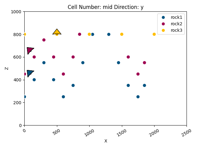
# Display a basic cross section of input data
gpv.plot_2d(geo_model)
<gempy_viewer.modules.plot_2d.visualization_2d.Plot2D object at 0x7f9a076e9fd0>
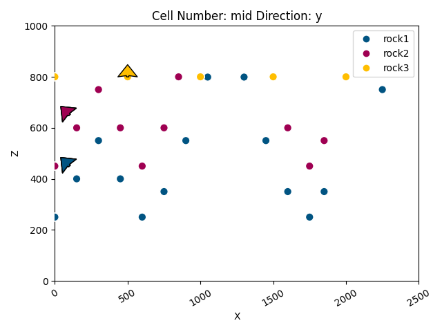
# Manually add a surface point
gp.add_surface_points(
    geo_model=geo_model,
    x=[2250],
    y=[500],
    z=[750],
    elements_names=['rock1']
)
# Show added point in cross section
gpv.plot_2d(geo_model)
<gempy_viewer.modules.plot_2d.visualization_2d.Plot2D object at 0x7f9a07439090>
Video tutorial 3: Structural frame
# View structural frame
geo_model.structural_frame
# View structural elements
geo_model.structural_frame.structural_elements
[Element(
    name=rock1,
    color=#015482,
    is_active=True
), Element(
    name=rock2,
    color=#9f0052,
    is_active=True
), Element(
    name=rock3,
    color=#ffbe00,
    is_active=True
), Element(
    name=basement,
    color=#728f02,
    is_active=True
)]
# Define structural groups and age/stratigraphic relationship
gp.map_stack_to_surfaces(
    gempy_model=geo_model,
    mapping_object={
        "Strat_Series2": ("rock3"),
        "Strat_Series1": ("rock2", "rock1")
    }
)
Video tutorial 4: Computation and results
# View interpolation options
geo_model.interpolation_options
InterpolationOptions(kernel_options=KernelOptions(range=1.7, c_o=10.0, uni_degree=1, i_res=4.0, gi_res=2.0, number_dimensions=3, kernel_function=AvailableKernelFunctions.cubic, kernel_solver=Solvers.DEFAULT, compute_condition_number=False, optimizing_condition_number=False, condition_number=None, condition_number_before=None, condition_number_after=None, fault_drift_equilibration=True, fault_drift_regularization=0.001, symmetric_equilibration_method=none, symmetric_equilibration_max_iterations=10, symmetric_equilibration_tolerance=0.01, nugget_implementation=NuggetImplementation.LEGACY, drift_diagnostics=False, drift_rank_policy=warn, drift_rank_rcond=None, drift_warning_rcond=None), evaluation_options=EvaluationOptions(_number_octree_levels=1, _number_octree_levels_surface=4, octree_curvature_threshold=-1.0, octree_error_threshold=1.0, octree_min_level=2, mesh_extraction=True, mesh_extraction_masking_options=<MeshExtractionMaskingOptions.INTERSECT: 3>, mesh_extraction_fancy=True, evaluation_chunk_size=500000, micro_anisotropic=MicroAnisotropicOptions(enabled=False, points=None, residuals=None, anisotropy_matrices=None, weights=None, kernel_range=1.0, kernel_type='matern_5_2', nugget=0.0, preserve_macro_points=True, strength=1.0), compute_scalar=True, compute_scalar_gradient=False, verbose=False), debug=False, cache_mode=<CacheMode.IN_MEMORY_CACHE: 3>, cache_model_name='tutorial_model', block_solutions_type=<BlockSolutionType.DENSE_GRID: 2>, sigmoid_slope=5000000)
# Compute a solution for the model
gp.compute_model(geo_model)
Setting Backend To: AvailableBackends.PYTORCH
GPU requested but unavailable; falling back to CPU (GEMPY_GPU_FALLBACK=True)
Setting Backend To: AvailableBackends.PYTORCH
Chunking done: 7 chunks
Chunking done: 30 chunks
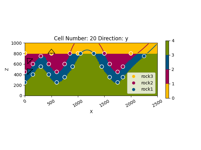
# Display the result in 2d section
gpv.plot_2d(geo_model, cell_number=20)
<gempy_viewer.modules.plot_2d.visualization_2d.Plot2D object at 0x7f9a0743ac10>
# Some examples of how to access results
print(geo_model.solutions.raw_arrays.lith_block)
print(geo_model.grid.dense_grid.values)
[4 4 4 ... 1 1 1]
[[  12.5   12.5   12.5]
 [  12.5   12.5   37.5]
 [  12.5   12.5   62.5]
 ...
 [2487.5  987.5  937.5]
 [2487.5  987.5  962.5]
 [2487.5  987.5  987.5]]
Video tutorial 5: 2D visualization
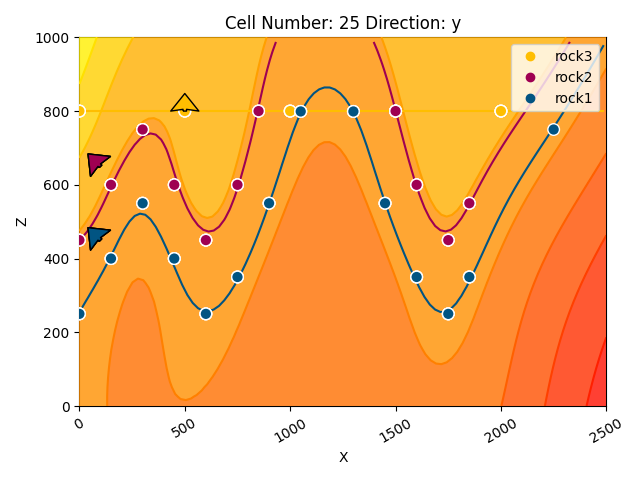
# 2d plotting options
gpv.plot_2d(geo_model, show_value=True, show_lith=False, show_scalar=True, series_n=1, cell_number=25)
<gempy_viewer.modules.plot_2d.visualization_2d.Plot2D object at 0x7f9a1a1f90f0>
# Create custom section lines
gp.set_section_grid(
    grid=geo_model.grid,
    section_dict={
        'section1': ([0, 0], [2500, 1000], [100, 50]),
        'section2': ([1000, 1000], [1500, 0], [100, 100]),
    }
)
Active grids: GridTypes.DENSE|SECTIONS|NONE
# Show custom cross-section traces
gpv.plot_section_traces(geo_model)
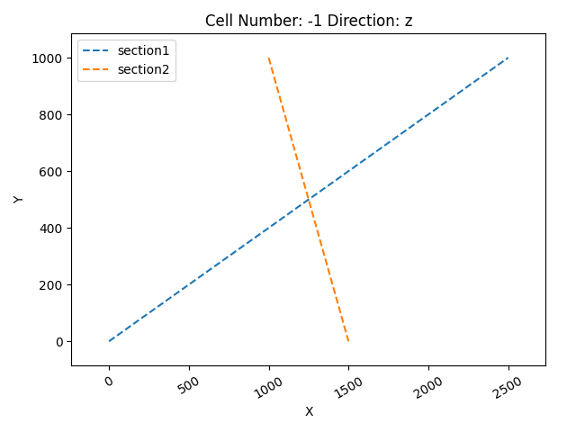
<function plot_section_traces at 0x7f9a105d8eb0>
# Recompute model as a new grid was added
gp.compute_model(geo_model)
Setting Backend To: AvailableBackends.PYTORCH
GPU requested but unavailable; falling back to CPU (GEMPY_GPU_FALLBACK=True)
Setting Backend To: AvailableBackends.PYTORCH
Chunking done: 8 chunks
Chunking done: 33 chunks
# Display custom cross-sections
gpv.plot_2d(geo_model, section_names=['section1', 'section2'], show_data=False)
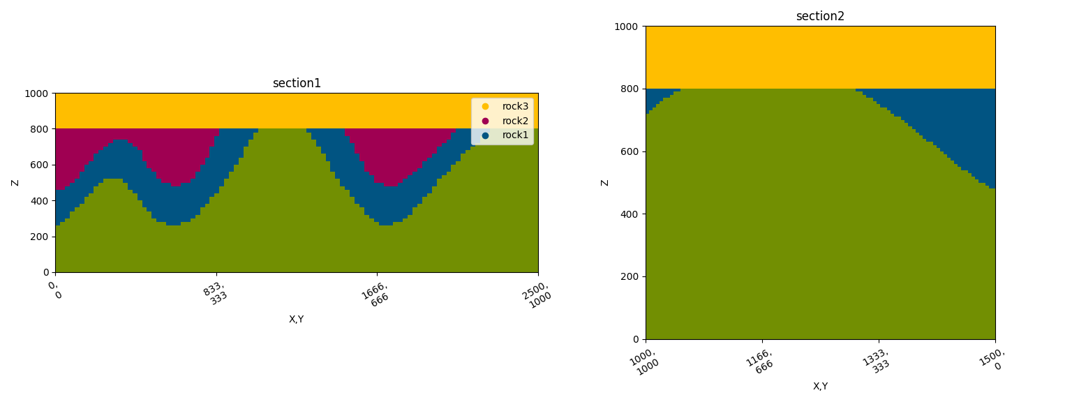
<gempy_viewer.modules.plot_2d.visualization_2d.Plot2D object at 0x7f9a19505b50>
Video tutorial 6: 3D visualization
# Display the result in 3d
gpv.plot_3d(geo_model, show_lith=True, show_boundaries=True, ve=None)
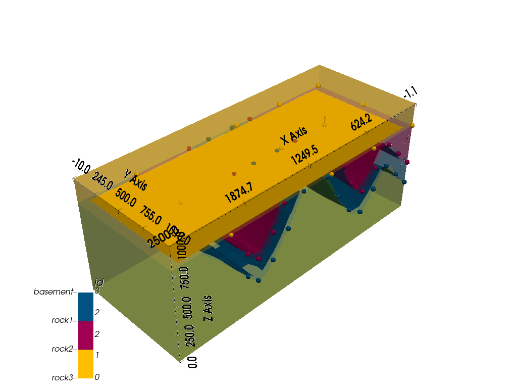
<gempy_viewer.modules.plot_3d.vista.GemPyToVista object at 0x7f9a07381e80>
Video tutorial 7: Topography
# Setting a randomly generated topography
import numpy as np

gp.set_topography_from_random(
    grid=geo_model.grid,
    fractal_dimension=1.2,
    d_z=np.array([700, 900]),
    topography_resolution=np.array([250, 100])
)
Active grids: GridTypes.DENSE|TOPOGRAPHY|SECTIONS|NONE

Topography(_regular_grid=RegularGrid(resolution=array([100,  40,  40]), extent=array([   0., 2500.,    0., 1000.,    0., 1000.]), values=array([[  12.5,   12.5,   12.5],
       [  12.5,   12.5,   37.5],
       [  12.5,   12.5,   62.5],
       ...,
       [2487.5,  987.5,  937.5],
       [2487.5,  987.5,  962.5],
       [2487.5,  987.5,  987.5]], shape=(160000, 3)), mask_topo=array([], shape=(0, 3), dtype=bool), _transform=None, _base_resolution=array([2, 2, 2])), values_2d=array([[[   0.        ,    0.        ,  806.5888454 ],
        [   0.        ,   10.1010101 ,  805.41476253],
        [   0.        ,   20.2020202 ,  804.27779025],
        ...,
        [   0.        ,  979.7979798 ,  724.75850286],
        [   0.        ,  989.8989899 ,  724.45465258],
        [   0.        , 1000.        ,  724.15136232]],

       [[  10.04016064,    0.        ,  806.00436567],
        [  10.04016064,   10.1010101 ,  804.81430883],
        [  10.04016064,   20.2020202 ,  803.61546993],
        ...,
        [  10.04016064,  979.7979798 ,  725.11489205],
        [  10.04016064,  989.8989899 ,  724.86314474],
        [  10.04016064, 1000.        ,  724.60767754]],

       [[  20.08032129,    0.        ,  805.37206419],
        [  20.08032129,   10.1010101 ,  804.24118234],
        [  20.08032129,   20.2020202 ,  803.03498538],
        ...,
        [  20.08032129,  979.7979798 ,  725.45855758],
        [  20.08032129,  989.8989899 ,  725.3067018 ],
        [  20.08032129, 1000.        ,  725.14014953]],

       ...,

       [[2479.91967871,    0.        ,  808.94931514],
        [2479.91967871,   10.1010101 ,  807.79223131],
        [2479.91967871,   20.2020202 ,  806.65075679],
        ...,
        [2479.91967871,  979.7979798 ,  723.9652805 ],
        [2479.91967871,  989.8989899 ,  723.57423016],
        [2479.91967871, 1000.        ,  723.14341083]],

       [[2489.95983936,    0.        ,  808.12494266],
        [2489.95983936,   10.1010101 ,  806.94502238],
        [2489.95983936,   20.2020202 ,  805.83830321],
        ...,
        [2489.95983936,  979.7979798 ,  724.16160672],
        [2489.95983936,  989.8989899 ,  723.80304682],
        [2489.95983936, 1000.        ,  723.39759727]],

       [[2500.        ,    0.        ,  807.3014964 ],
        [2500.        ,   10.1010101 ,  806.12348615],
        [2500.        ,   20.2020202 ,  805.01636651],
        ...,
        [2500.        ,  979.7979798 ,  724.43139443],
        [2500.        ,  989.8989899 ,  724.12131066],
        [2500.        , 1000.        ,  723.76706711]]],
      shape=(250, 100, 3)), source=None, values=array([[   0.        ,    0.        ,  806.5888454 ],
       [   0.        ,   10.1010101 ,  805.41476253],
       [   0.        ,   20.2020202 ,  804.27779025],
       ...,
       [2500.        ,  979.7979798 ,  724.43139443],
       [2500.        ,  989.8989899 ,  724.12131066],
       [2500.        , 1000.        ,  723.76706711]], shape=(25000, 3)), resolution=(250, 100), raster_shape=())
# Recompute model as a new grid was added
gp.compute_model(geo_model)
Setting Backend To: AvailableBackends.PYTORCH
GPU requested but unavailable; falling back to CPU (GEMPY_GPU_FALLBACK=True)
Setting Backend To: AvailableBackends.PYTORCH
Chunking done: 9 chunks
Chunking done: 37 chunks
# Display a cross-section with topography
gpv.plot_2d(geo_model, show_topography=True)
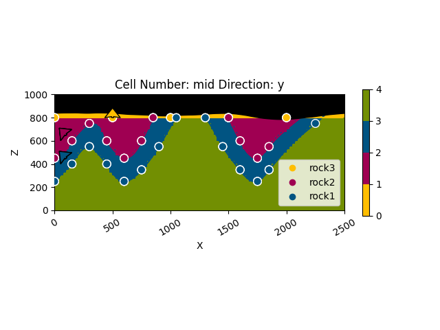
<gempy_viewer.modules.plot_2d.visualization_2d.Plot2D object at 0x7f9a07546030>
# Displaying a geological map
gpv.plot_2d(geo_model, show_topography=True, section_names=['topography'], show_boundaries=False, show_data=False)
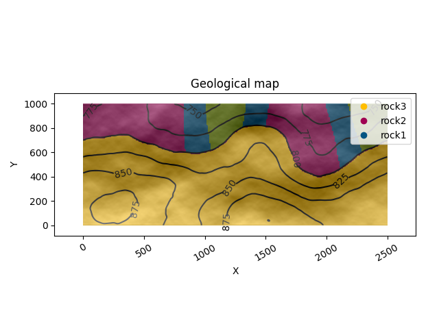
<gempy_viewer.modules.plot_2d.visualization_2d.Plot2D object at 0x7f9a073e47c0>
# Display the 3d model with topography
gpv.plot_3d(geo_model, show_lith=True, show_topography=True)

# sphinx_gallery_thumbnail_number = -1
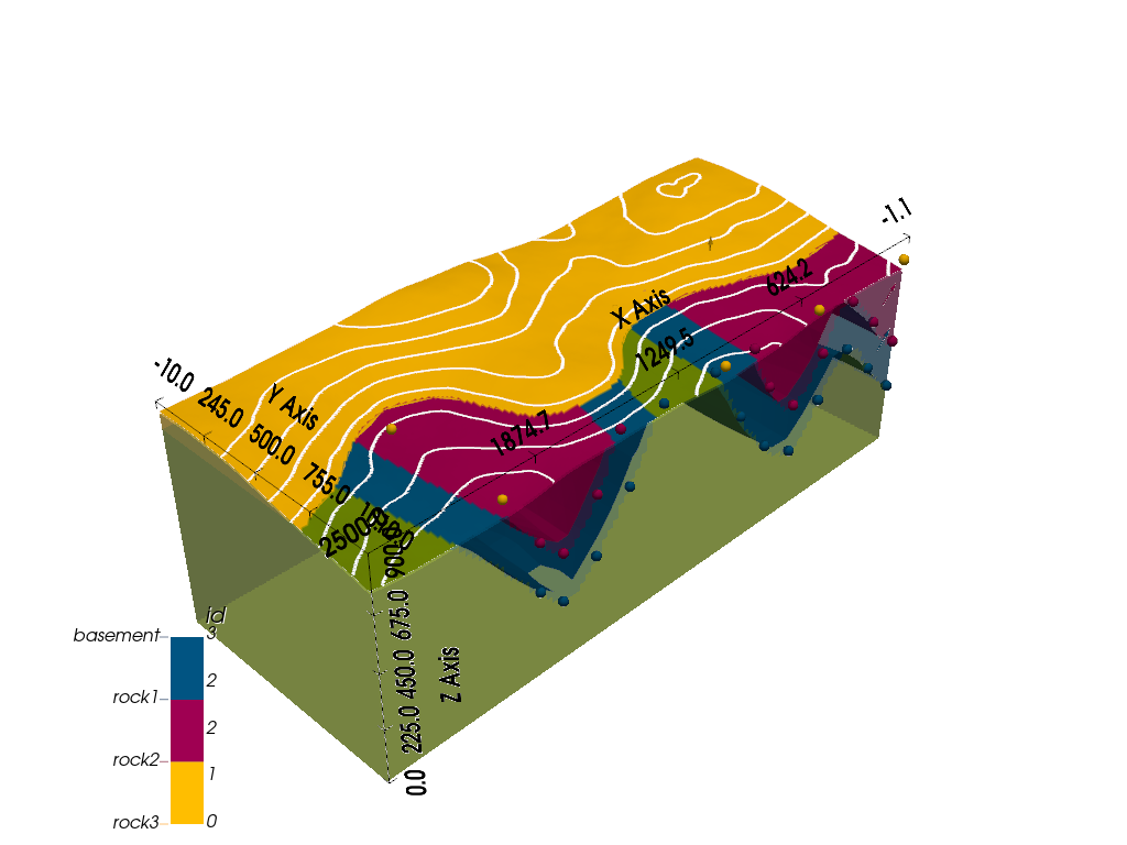
<gempy_viewer.modules.plot_3d.vista.GemPyToVista object at 0x7f9a29e6e5d0>
Total running time of the script: (0 minutes 20.050 seconds)