1.3a: Grids.

import numpy as np
import matplotlib.pyplot as plt

import gempy as gp
from gempy.core.data import Grid

np.random.seed(55500)

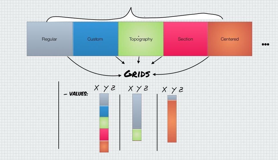
The Grid Class

The grid class will interact with the rest of data classes and grid subclasses. Its main purpose is to feed coordinates XYZ to the interpolator.

grid = Grid()

The most important attribute of Grid is values (and values_r which are the values rescaled) which are the 3D points in space that kriging will be evaluated on. This array will be feed by “grid types” on a composition relation with Grid:

grid.values, grid.values_r

(array([], shape=(0, 3), dtype=float64), array([], shape=(0, 3), dtype=float64))

At the moment of writing this tutorial, there is 5 grid types. The number of grid types is scalable and down the road we aim to connect other grid packages (like Discretize) as an extra Grid type

grid.grid_types

array(['regular', 'custom', 'topography', 'sections', 'centered',
       'octree'], dtype='<U10')

Each grid contains its own values attribute as well as other methods to manipulate them depending on the type of grid.

grid.values

array([], shape=(0, 3), dtype=float64)

We can see what grids are activated (i.e. they are going to be interpolated and therefore will live on Grid().values) by:

grid.active_grids_bool

array([False, False, False, False, False, False])

By default only the regular grid (grid.regular_grid) is active. However, since the regular grid is still empty Grid().values is empty too.

grid.values

array([], shape=(0, 3), dtype=float64)

The last important attribute of Grid is the length:

grid.length

array([0, 0, 0, 0, 0, 0])

Length gives back the interface indices between grids on the Grid().values attribute. This can be used after interpolation to know which interpolated values and coordinates correspond to each grid type. You can use the method get_grid_args to return the indices by name:

grid.get_grid_args('topography')

(0, 0)

By now all is a bit confusing because we have no values. Lets start adding values to the different grids:

Regular grid

The Grid class has a bunch of methods to set each grid type and activate them.

help(grid.create_regular_grid)

Help on method create_regular_grid in module gempy.core.data.grid:

create_regular_grid(extent=None, resolution=None, set_active=True, *args, **kwargs) method of gempy.core.data.grid.Grid instance
    Set a new regular grid and activate it.

    Args:
        extent (np.ndarray): [x_min, x_max, y_min, y_max, z_min, z_max]
        resolution (np.ndarray): [nx, ny, nz]

    RegularGrid Docs

grid.create_regular_grid(extent=[0, 100, 0, 100, -100, 0], resolution=[20, 20, 20])

<gempy.core.data.grid_modules.grid_types.RegularGrid object at 0x7f49496d0b20>

Now the regular grid object composed on Grid has been filled:

grid.regular_grid.values

array([[  2.5,   2.5, -97.5],
       [  2.5,   2.5, -92.5],
       [  2.5,   2.5, -87.5],
       ...,
       [ 97.5,  97.5, -12.5],
       [ 97.5,  97.5,  -7.5],
       [ 97.5,  97.5,  -2.5]])

And the regular grid has been set active (it was already active in any case):

grid.active_grids_bool

array([False, False, False, False, False, False])

Therefore the grid values will be equal to the regular grid:

grid.values

array([], shape=(0, 3), dtype=float64)

And the indices to extract the different arrays:

grid.length

array([0, 0, 0, 0, 0, 0])

Custom grid

Completely free XYZ values.

gp.set_custom_grid(grid, np.array([[1, 2, 3], [4, 5, 6], [7, 8, 9]]))

Active grids: ['custom']

<gempy.core.data.grid_modules.grid_types.CustomGrid object at 0x7f49496d0df0>

Again set_any_grid will create a grid and activate it. So now the compose object will contain values:

grid.custom_grid.values

array([[1, 2, 3],
       [4, 5, 6],
       [7, 8, 9]])

and since it is active, will be added to the grid.values stack:

grid.active_grids_bool

array([False,  True, False, False, False, False])

grid.values.shape

(0, 3)

We can still recover those values with get_grid or by getting the slicing args:

grid.get_grid('custom')

array([], shape=(0, 3), dtype=float64)

l0, l1 = grid.get_grid_args('custom')
l0, l1

(0, 0)

grid.values[l0:l1]

array([], shape=(0, 3), dtype=float64)

Topography

Now we can set the topography. Topography contains methods to create manual topographies as well as gdal for dealing with raster data. By default we will create a random topography:

gp.set_topography_from_random(grid)

[-20.   0.]
Active grids: ['custom' 'topography']

<gempy.core.data.grid_modules.topography.Topography object at 0x7f4949769690>

grid.active_grids_bool

array([False,  True,  True, False, False, False])

Now the grid values will contain both the regular grid and topography:

grid.values, grid.length

(array([], shape=(0, 3), dtype=float64), array([0, 0, 0, 0, 0, 0]))

The topography args are got as follows:

l0, l1 = grid.get_grid_args('topography')
l0, l1

(0, 0)

And we can slice the values array as any other numpy array:

grid.values[l0: l1]

array([], shape=(0, 3), dtype=float64)

We can compare it to the topography.values:

grid.topography.values

array([[  0.        ,   0.        , -14.23224119],
       [  0.        ,   5.26315789, -14.18893341],
       [  0.        ,  10.52631579, -13.54018217],
       ...,
       [100.        ,  89.47368421, -14.13839552],
       [100.        ,  94.73684211, -16.12793911],
       [100.        , 100.        , -16.21462612]])

Now that we have more than one grid we can activate and deactivate any of them in real time:

grid.set_inactive('topography')
grid.set_inactive('regular')

array([False,  True, False, False, False, False])

Since now all grids are deactivated the values will be empty:

grid.values

array([[1., 2., 3.],
       [4., 5., 6.],
       [7., 8., 9.]])

grid.set_active('topography')

array([False,  True,  True, False, False, False])

grid.values, grid.values.shape

(array([[  1.        ,   2.        ,   3.        ],
       [  4.        ,   5.        ,   6.        ],
       [  7.        ,   8.        ,   9.        ],
       ...,
       [100.        ,  89.47368421, -14.13839552],
       [100.        ,  94.73684211, -16.12793911],
       [100.        , 100.        , -16.21462612]]), (403, 3))

grid.set_active('regular')

array([ True,  True,  True, False, False, False])

grid.values

array([[  2.5       ,   2.5       , -97.5       ],
       [  2.5       ,   2.5       , -92.5       ],
       [  2.5       ,   2.5       , -87.5       ],
       ...,
       [100.        ,  89.47368421, -14.13839552],
       [100.        ,  94.73684211, -16.12793911],
       [100.        , 100.        , -16.21462612]])

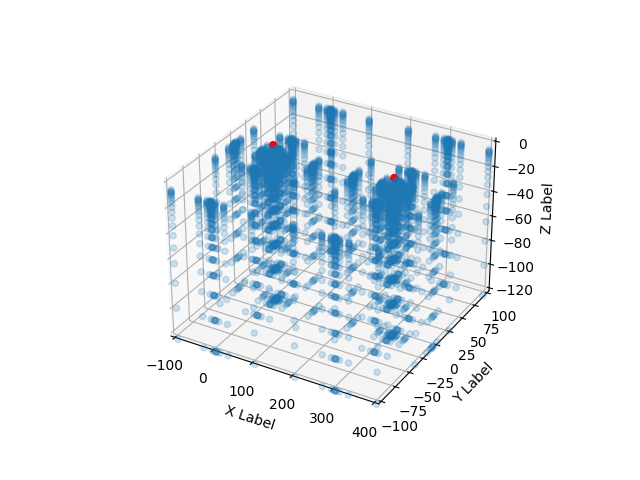
Centered Grid

This grid contains an irregular grid where the majority of voxels are centered around a value (or values). This type of grid is usually used to compute certain types of forward physics where the influence decreases with distance (e.g. gravity: Check tutorial 2.2-Cell-selection )

gp.set_centered_grid(
    grid,
    centers=np.array([[300, 0, 0], [0, 0, 0]]),
    resolution=[10, 10, 20],
    radius=np.array([100, 100, 100])
)

Active grids: ['regular' 'custom' 'topography' 'centered']

CenteredGrid(centers=array([[300,   0,   0],
       [  0,   0,   0]]), resolution=[10, 10, 20], radius=array([100, 100, 100]), kernel_grid_centers=array([[-100.        , -100.        ,   -6.        ],
       [-100.        , -100.        ,   -7.2       ],
       [-100.        , -100.        ,   -7.52912998],
       ...,
       [ 100.        ,  100.        ,  -79.90178533],
       [ 100.        ,  100.        , -100.17119644],
       [ 100.        ,  100.        , -126.        ]]), left_voxel_edges=array([[ 34.1886117 ,  34.1886117 ,  -0.6       ],
       [ 34.1886117 ,  34.1886117 ,  -0.6       ],
       [ 34.1886117 ,  34.1886117 ,  -0.16456499],
       ...,
       [ 34.1886117 ,  34.1886117 ,  -7.95331123],
       [ 34.1886117 ,  34.1886117 , -10.13470556],
       [ 34.1886117 ,  34.1886117 , -12.91440178]]), right_voxel_edges=array([[ 34.1886117 ,  34.1886117 ,  -0.6       ],
       [ 34.1886117 ,  34.1886117 ,  -0.16456499],
       [ 34.1886117 ,  34.1886117 ,  -0.20970105],
       ...,
       [ 34.1886117 ,  34.1886117 , -10.13470556],
       [ 34.1886117 ,  34.1886117 , -12.91440178],
       [ 34.1886117 ,  34.1886117 , -12.91440178]]))

Resolution and radius create a geometric spaced kernel (blue dots) which will be use to create a grid around each of the center points (red dots):

fig = plt.figure()
ax = fig.add_subplot(111, projection='3d')

ax.scatter(
    grid.centered_grid.values[:, 0],
    grid.centered_grid.values[:, 1],
    grid.centered_grid.values[:, 2],
    '.',
    alpha=.2
)

ax.scatter(
    np.array([[300, 0, 0], [0, 0, 0]])[:, 0],
    np.array([[300, 0, 0], [0, 0, 0]])[:, 1],
    np.array([[300, 0, 0], [0, 0, 0]])[:, 2],
    c='r',
    alpha=1,
    s=30
)

ax.set_xlim(-100, 400)
ax.set_ylim(-100, 100)
ax.set_zlim(-120, 0)
ax.set_xlabel('X Label')
ax.set_ylabel('Y Label')
ax.set_zlabel('Z Label')
plt.show()

Section Grid

This grid type has its own tutorial. See :doc: ch1_3b_cross_sections