Note
Go to the end to download the full example code.
1.1 -Basics of geological modeling with GemPy
import numpy as np
Importing Necessary Libraries
import gempy as gp
import gempy_viewer as gpv
Importing and Defining Input Data
gempy.core.data.GeoModel
GemPy uses Python objects to store the data that builds the geological model. The main data classes include:
You can also create data from raw CSV files (comma-separated values). This could be useful if you are exporting model data from a different program or creating it in a spreadsheet software like Microsoft Excel or LibreOffice Calc.
In this tutorial, we’ll use CSV files to generate input data. You can find these example files in the gempy data repository on GitHub. The data consists of x, y, and z positional values for all surface points and orientation measurements. Additional data includes poles, azimuth and polarity (or the gradient components). Surface points are assigned a formation, which can be a lithological unit (like “Sandstone”) or a structural feature (like “Main Fault”).
It’s important to note that, in GemPy, interface position points mark the bottom of a layer. If you need points to represent the top of a formation (for example, when modeling an intrusion), you can define an inverted orientation measurement.
While generating data from CSV files, we also need to define the model’s real extent in x, y, and z. This extent defines the area used for interpolation and many of the plotting functions. We also set a resolution to establish a regular grid right away. This resolution will dictate the number of voxels used during modeling. We’re using a medium resolution of 50x50x50 here, which results in 125,000 voxels. The model extent should enclose all relevant data in a representative space. As our model voxels are prisms rather than cubes, the resolution can differ from the extent. However, it is recommended to avoid going beyond 100 cells in each direction (1,000,000 voxels) to prevent excessive computational costs.
data_path = 'https://raw.githubusercontent.com/cgre-aachen/gempy_data/master/'

geo_model: gp.data.GeoModel = gp.create_geomodel(
    project_name='Tutorial_ch1_1_Basics',
    extent=[0, 2000, 0, 2000, 0, 750],
    refinement=6,  # * Here we define the number of octree levels. If octree levels are defined, the resolution is ignored.
    importer_helper=gp.data.ImporterHelper(
        path_to_orientations=data_path + "/data/input_data/getting_started/simple_fault_model_orientations.csv",
        path_to_surface_points=data_path + "/data/input_data/getting_started/simple_fault_model_points.csv",
        hash_surface_points="4cdd54cd510cf345a583610585f2206a2936a05faaae05595b61febfc0191563",
        hash_orientations="7ba1de060fc8df668d411d0207a326bc94a6cdca9f5fe2ed511fd4db6b3f3526"
    )
)
Surface points hash:  4cdd54cd510cf345a583610585f2206a2936a05faaae05595b61febfc0191563
Orientations hash:  7ba1de060fc8df668d411d0207a326bc94a6cdca9f5fe2ed511fd4db6b3f3526
New in GemPy 3!
GemPy 3 has introduced the ImporterHelper class to streamline importing data from various sources. This class
simplifies the process of passing multiple arguments needed for importing data and will likely see further
extensions in the future. Currently, one of its uses is to handle pooch arguments for downloading data from the internet.
Reviewing the Imported Data
Now that the geo_model object is set up and the data imported from the CSV files, we review the data imported using the properties surface_points_copy and orientations_copy.
Using structural_frame.element_id_name_map, we can see which ID corresponds to which structural element name in the data.
Declaring the Sequential Order of Structural Elements (Geological Formations)
In our model, we want the geological units to appear in the correct chronological order. This order could be determined by a sequence of stratigraphic deposition, unconformities due to erosion, or other lithological genesis events like igneous intrusions. A similar age-related order is declared for faults in our model. In GemPy, we use the function gempy.map_stack_to_surfaces to assign formations or faults to different sequential series by declaring them in a Python dictionary.
The correct ordering of series is crucial for model construction! It’s possible to assign several surfaces to one series. The order of units within a series only affects the color code, so we recommend maintaining consistency. The order can be defined by simply changing the order of the lists within the gempy.core.data.StructuralFrame.structural_groups and gempy.core.data.StructuralGroups.elements attributes.
Faults are treated as independent groups and must be younger than the groups they affect. The relative order between different faults defines their tectonic relationship (the first entry is the youngest).
For a model with simple sequential stratigraphy, all layer formations can be assigned to one series without an issue. All unit boundaries and their order would then be determined by interface points. However, to model more complex lithostratigraphical relations and interactions, separate series definitions become important. For example, modeling an unconformity or an intrusion that disrupts older stratigraphy would require declaring a younger series.
By default, a simple sequence/group is created inferred from the data as shown above.
Our example model comprises four main layers (plus an underlying basement that is automatically generated by GemPy) and one main normal fault displacing those layers. Assuming a simple stratigraphy where each younger unit was deposited onto the underlying older one, we can assign these layer formations to one structural group called “Strat_Series”. For the fault, we declare a respective “Fault_Series” as the first key entry in the mapping dictionary. We could give any other names to these series; the formations, however, have to be referred to as named in the input data.
In the following, we map the “Main Fault” to the “Fault Series” and the individual formations to the “Strat Series”.
gp.map_stack_to_surfaces(
    gempy_model=geo_model,
    mapping_object=  # TODO: This mapping I do not like it too much. We should be able to do it passing the data objects directly
    {
            "Fault_Series": 'Main_Fault',
            "Strat_Series": ('Sandstone_2', 'Siltstone', 'Shale', 'Sandstone_1')
    }
)
Note how the structural frame still indicates the “Fault Series” group to have a relation type “erode”. We still need to tell GemPy that we want this group to be a fault. We do this using the function set_is_fault.
gp.set_is_fault(
    frame=geo_model.structural_frame,
    fault_groups=['Fault_Series']
)
Now, all surfaces have been assigned to a series and are displayed in the correct order (from young to old).
Returning Information from Our Input Data
Our model input data, named “geo_model”, contains all essential information for constructing our model. You can access different types of information by accessing the attributes. For instance, you can retrieve the coordinates of our modeling grid as follows:
Grid(values=array([[   5.20833333,    5.20833333,    5.859375  ],
       [   5.20833333,    5.20833333,   17.578125  ],
       [   5.20833333,    5.20833333,   29.296875  ],
       ...,
       [1994.79166667, 1994.79166667,  720.703125  ],
       [1994.79166667, 1994.79166667,  732.421875  ],
       [1994.79166667, 1994.79166667,  744.140625  ]], shape=(2359296, 3)), length=array([], dtype=float64), _octree_grid=RegularGrid(resolution=array([192, 192,  64]), extent=array([   0., 2000.,    0., 2000.,    0.,  750.]), values=array([[   5.20833333,    5.20833333,    5.859375  ],
       [   5.20833333,    5.20833333,   17.578125  ],
       [   5.20833333,    5.20833333,   29.296875  ],
       ...,
       [1994.79166667, 1994.79166667,  720.703125  ],
       [1994.79166667, 1994.79166667,  732.421875  ],
       [1994.79166667, 1994.79166667,  744.140625  ]], shape=(2359296, 3)), mask_topo=array([], shape=(0, 3), dtype=bool), _transform=None, _base_resolution=array([6, 6, 2])), _dense_grid=None, _custom_grid=None, _topography=None, _sections=None, _centered_grid=None, _transform=None, _octree_levels=-1)
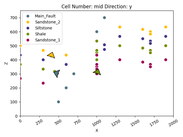
Visualizing input data
Since we have already imported our input data, we can go ahead and visualize it in 2D and 3D. This can be useful to check if all points and orientations are defined the way we want them to be. Using the function gempy_viewer.plot2d, we obtain a 2D projection of our data points onto a plane of the chosen direction (we can choose this attribute to be either x, y or z, with the default being y). Below, we can freely switch the direction and check out the projection from different sides to get a good idea.
plot = gpv.plot_2d(geo_model, show_lith=False, show_boundaries=False)
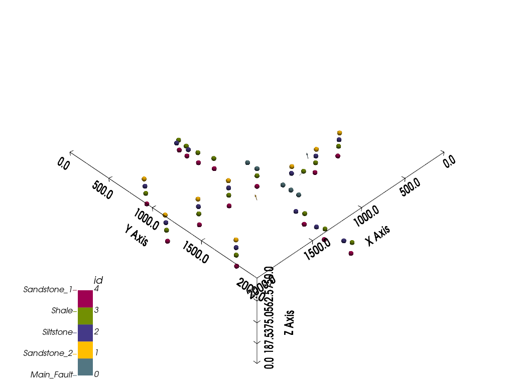
Beyond 2D, however, we can also visualize our input data in full 3D using gempy_viewer.plot_3d. Note that direct 3D visualization in GemPy requires [the Visualization Toolkit](https://www.vtk.org/) (VTK) to be installed.
gpv.plot_3d(geo_model, image=False, plotter_type='basic')
<gempy_viewer.modules.plot_3d.vista.GemPyToVista object at 0x7f58217b39b0>
Model Generation
Once we’ve correctly defined all our primary information in our gempy.core.data.GeoModel object (referred to as geo_model in these tutorials), we can proceed with the model computation step. We can go ahead and save the solution of a specific computation as we do below, but solutions are also stored within the gempy.core.data.GeoModel object for future reference.
New in GemPy 3! Numpy and TensorFlow backend
Unlike previous versions, GemPy 3 doesn’t rely on theano or asera. Instead, it utilizes numpy or tensorflow. Consequently, we no longer need to recompile all theano functions (TensorFlow uses eager execution; we found no notable speed difference after profiling the XLA compiler).
The parameters used for the interpolation are stored in gempy.core.data.GeoModel.interpolation_options. These parameters have sensible default values that you can modify if necessary. However, we advise caution when changing these parameters unless you fully understand their implications.
Display the current interpolation options
geo_model.interpolation_options
InterpolationOptions(kernel_options=KernelOptions(range=1.7, c_o=10.0, uni_degree=1, i_res=4.0, gi_res=2.0, number_dimensions=3, kernel_function=AvailableKernelFunctions.cubic, kernel_solver=Solvers.DEFAULT, compute_condition_number=False, optimizing_condition_number=False, condition_number=None), evaluation_options=EvaluationOptions(_number_octree_levels=6, _number_octree_levels_surface=4, octree_curvature_threshold=-1.0, octree_error_threshold=1.0, octree_min_level=2, mesh_extraction=True, mesh_extraction_masking_options=<MeshExtractionMaskingOptions.INTERSECT: 3>, mesh_extraction_fancy=True, evaluation_chunk_size=500000, compute_scalar=True, compute_scalar_gradient=False, verbose=False), debug=False, cache_mode=<CacheMode.IN_MEMORY_CACHE: 3>, cache_model_name='Tutorial_ch1_1_Basics', block_solutions_type=<BlockSolutionType.OCTREE: 1>, sigmoid_slope=5000000)
With all our prerequisites in place, we can now compute our complete geological model
using gempy.compute_model(). This function returns a gempy.core.data.Solutions object.
The following sections illustrate these different model solutions and how to utilize them.
Compute the geological model and get the solutions
sol = gp.compute_model(geo_model)
sol
Setting Backend To: AvailableBackends.PYTORCH
GPU requested but unavailable; falling back to CPU (GEMPY_GPU_FALLBACK=True)
Setting Backend To: AvailableBackends.PYTORCH
Chunking done: 18 chunks
Chunking done: 16 chunks
Chunking done: 89 chunks
Chunking done: 7 chunks
Chunking done: 41 chunks
Chunking done: 7 chunks
Solutions are also stored within the gempy.core.data.GeoModel object, for future reference.
geo_model.solutions
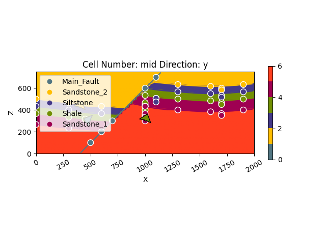
Direct model visualization in GemPy
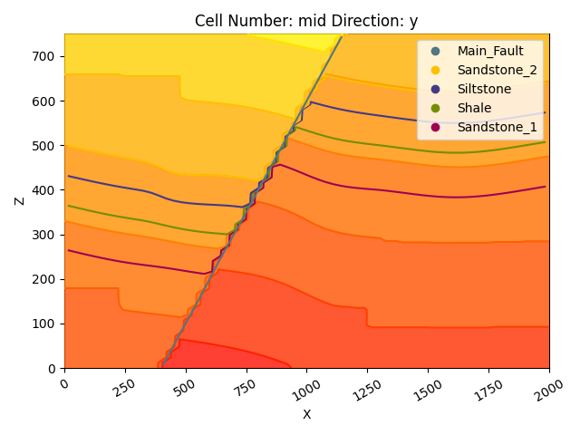
Model solutions can be easily visualized in 2D sections in GemPy directly. Let’s take a look at our lithology block:
gpv.plot_2d(geo_model, show_data=True, cell_number="mid", direction='y')
<gempy_viewer.modules.plot_2d.visualization_2d.Plot2D object at 0x7f57bff4f540>
With cell_number=mid, we have chosen a section going through
the middle of our block. We have moved in direction='y',
the plot thus depicts a plane parallel to the \(x\)- and
\(y\)-axes. Setting show_data=True, we could plot original data
together with the results. Changing the values for cell_number and
direction, we can move through our 3D block model and explore it by
looking at different 2D planes.
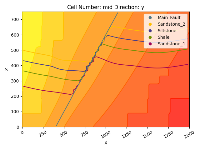
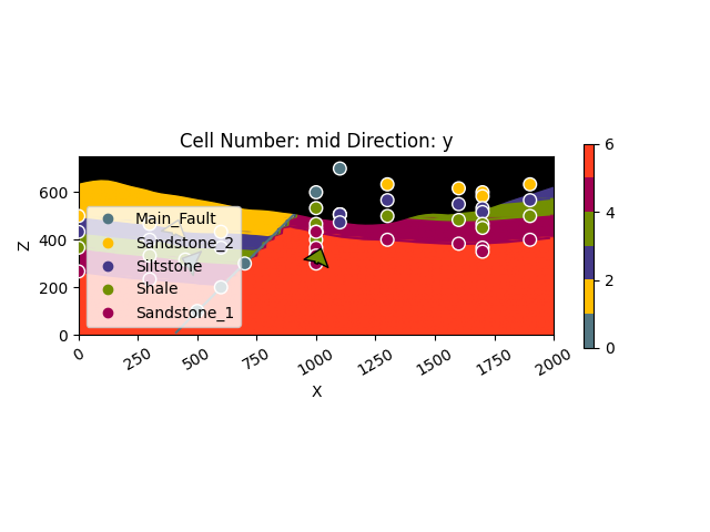
We can do the same with the underlying scalar-field solution:
gpv.plot_2d(
    model=geo_model,
    series_n=0,  # This will plot the scalar field used for the fault
    show_data=False,
    show_scalar=True,
    show_lith=False
)
<gempy_viewer.modules.plot_2d.visualization_2d.Plot2D object at 0x7f5820625630>
gpv.plot_2d(
    model=geo_model,
    series_n=1,  # This will plot the scalar field used for the stratigraphy
    show_data=False,
    show_scalar=True,
    show_lith=False
)
<gempy_viewer.modules.plot_2d.visualization_2d.Plot2D object at 0x7f5820dce990>
Dual Contouring and vtk visualization
In addition to 2D sections we can extract surfaces to visualize in 3D
renderers. Surfaces can be visualized as 3D triangle complexes in VTK
(see function plot_surfaces_3D below). To create these triangles, we
need to extract respective vertices and simplices from the potential
fields of lithologies and faults. This process is automatized in GemPy
using dual contouring in the gempy_engine.
New in GemPy 3! Dual Contouring
GemPy 3 uses dual contouring to extract surfaces from the scalar fields. The method is completely coded in gempy_engine what also
enables further improvements in the midterm. This method is more efficient to use
together with octrees and suited better the new capabilities of gempy3.
gpv.plot_3d(geo_model, show_data=False, image=False, plotter_type='basic')
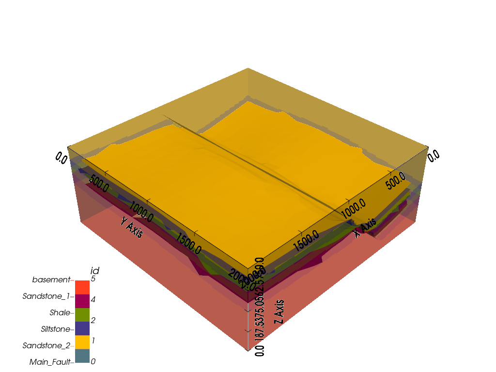
<gempy_viewer.modules.plot_3d.vista.GemPyToVista object at 0x7f58217fad50>
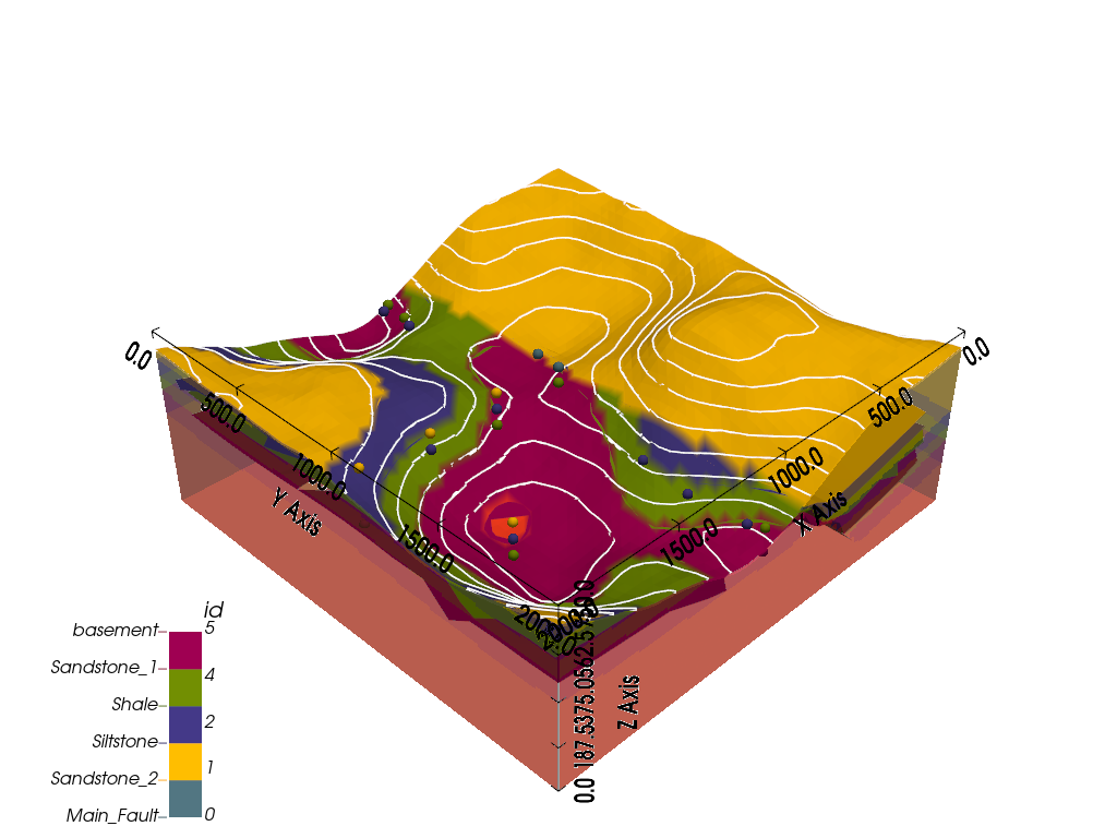
Adding topography
In gempy we can add more grid types for different purposes. We will explore this concept in more detail in the next tutorials (1.3a: Grids.). For now, we will just add a topography grid to our model. This grid allows us to intersect the surfaces as well as compute a high resolution geological mal.
gp.set_topography_from_random(
    grid=geo_model.grid,
    fractal_dimension=1.2,
    d_z=np.array([350, 750]),
    topography_resolution=np.array([50, 50]),
)

gp.compute_model(geo_model)
gpv.plot_2d(geo_model, show_topography=True)

gpv.plot_3d(
    model=geo_model,
    plotter_type='basic',
    show_topography=True,
    show_surfaces=True,
    show_lith=True,
    image=False
)
Active grids: GridTypes.OCTREE|TOPOGRAPHY|NONE
Setting Backend To: AvailableBackends.PYTORCH
GPU requested but unavailable; falling back to CPU (GEMPY_GPU_FALLBACK=True)
Setting Backend To: AvailableBackends.PYTORCH
Chunking done: 18 chunks
Chunking done: 16 chunks
Chunking done: 89 chunks
Chunking done: 7 chunks
Chunking done: 41 chunks
Chunking done: 7 chunks

<gempy_viewer.modules.plot_3d.vista.GemPyToVista object at 0x7f58217fa750>
Compute at a given location
This is done by modifying the grid to a custom grid and recomputing.
x_i = np.array([[1000, 1000, 1000]])
lith_values_at_coords: np.ndarray = gp.compute_model_at(
    gempy_model=geo_model,
    at=x_i
)
lith_values_at_coords
WARNING: This function sets a custom grid and computes the model so be wary of side effects.
Active grids: GridTypes.CUSTOM|NONE
Setting Backend To: AvailableBackends.PYTORCH
GPU requested but unavailable; falling back to CPU (GEMPY_GPU_FALLBACK=True)
Setting Backend To: AvailableBackends.PYTORCH
Chunking done: 18 chunks
Chunking done: 16 chunks
Chunking done: 89 chunks
Chunking done: 7 chunks
Chunking done: 41 chunks
Chunking done: 7 chunks

array([2.])
Therefore if we just want the value at x_i:
geo_model.solutions.raw_arrays.custom
array([2.])
Work in progress
GemPy3 model serialization is currently being redisigned. Therefore, at the current version, there is not a build in
method to save the model. However, since now the data model should be completely robust, you should be able to save the
gempy.core.data.GeoModel and all its attributes using the standard python library [pickle](https://docs.python.org/3/library/pickle.html)
sphinx_gallery_thumbnail_number = -2
Total running time of the script: (0 minutes 33.480 seconds)