Analyzing Geomodel Topology

Extracting adjacency graphs and topology relationships from a computed model

This tutorial uses the gempy_plugins topology analysis module to derive an adjacency graph between the unique geobodies of a faulted model, then visualizes and queries that graph.

Note

This tutorial relies on gempy_plugins, a separate package maintained in its own repository rather than by the core GemPy developers.

import gempy as gp
import gempy_viewer as gpv
from gempy_plugins.topology_analysis import topology as tp

import os

import warnings
warnings.filterwarnings("ignore")

Load example Model

First let’s set up a very simple example model. For that we initialize the geo_model object with the correct model extent and the resolution we like. Then we load our data points from csv files and set the series and order the formations (stratigraphic pile).

data_path = os.path.abspath('../../')

geo_model = gp.create_geomodel(
    project_name='Model_Tutorial6',
    extent=[0, 3000, 0, 20, 0, 2000],
    resolution=[50, 10, 67],
    refinement=1,  # * For this model is better not to use octrees because we want to see what is happening in the scalar fields
    importer_helper=gp.data.ImporterHelper(
        path_to_orientations=data_path + "/data/input_data/tut_chapter6/ch6_data_fol.csv",
        path_to_surface_points=data_path + "/data/input_data/tut_chapter6/ch6_data_interf.csv",
    )
)

gp.map_stack_to_surfaces(
    gempy_model=geo_model,
    mapping_object=
    {
        "fault": "Fault",
        "Rest": ('Layer 2', 'Layer 3', 'Layer 4', 'Layer 5')
    }
)

gp.set_is_fault(geo_model, ['fault'])

geo_model.interpolation_options.mesh_extraction = False
gp.compute_model(geo_model)

Setting Backend To: AvailableBackends.PYTORCH
GPU enabled. Using device: cuda
GPU device count: 1
Current GPU device: 0

gpv.plot_2d(geo_model, cell_number=[5])

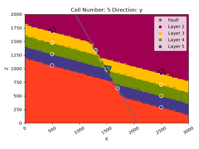
<gempy_viewer.modules.plot_2d.visualization_2d.Plot2D object at 0x7f3eea273450>

Analyzing Topology

The gempy_plugins topology module lets us analyze the topology of a model. All we need for this is our geo_model object, the lithology block, and the fault block. We pass those into tp.compute_topology, which is the starting point for several useful things:

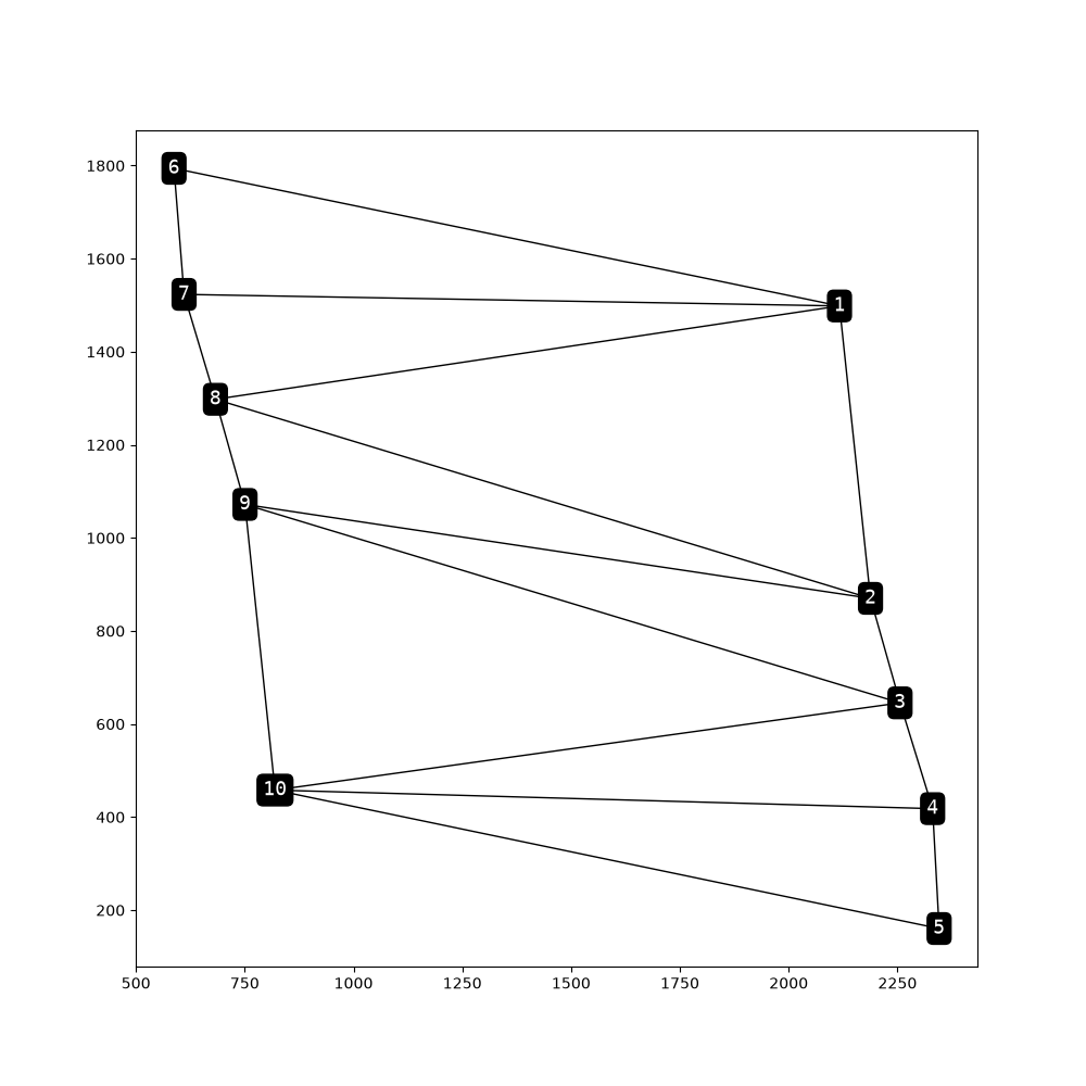
• an adjacency graph G, representing the topological relationships of the model

• the centroids of all the unique topological regions in the model (x,y,z coordinates of their center)

• from these, look-up tables between lithology id’s and node labels (and vice versa), and adjacency queries between specific geobodies

edges, centroids = tp.compute_topology(geo_model)

The first output of the topology function is the set of edges representing topology relationships between unique geobodies of the block model. An edge is represented by a tuple of two int geobody (or node) labels:

edges

{(9, 10), (4, 10), (1, 2), (3, 4), (1, 8), (3, 10), (2, 3), (2, 9), (1, 7), (4, 5), (3, 9), (5, 10), (6, 7), (8, 9), (1, 6), (7, 8), (2, 8)}

The second output is the centroids dict, mapping the unique geobody id’s (graph node id’s) to the geobody centroid position in grid coordinates:

centroids

{np.int64(1): array([35.27893175,  4.5       , 50.19485658]), np.int64(2): array([36.46666667,  4.5       , 29.14444444]), np.int64(3): array([37.59756098,  4.5       , 21.62195122]), np.int64(4): array([38.84563758,  4.5       , 14.00671141]), np.int64(5): array([39.09550562,  4.5       ,  5.37640449]), np.int64(6): array([ 9.79081633,  4.5       , 60.10204082]), np.int64(7): array([10.17687075,  4.5       , 51.02721088]), np.int64(8): array([11.37804878,  4.5       , 43.47560976]), np.int64(9): array([12.51098901,  4.5       , 35.90659341]), np.int64(10): array([13.659857  ,  4.5       , 15.34320735])}

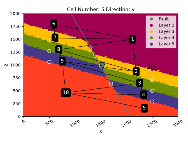
After computing the model topology, we can overlay the topology graph over a model section:

Visualizing topology

2-D Visualization of the Topology Graph

gpv.plot_topology(
    regular_grid=geo_model.grid.regular_grid,
    edges=edges,
    centroids=centroids
)

plot_2d = gpv.plot_2d(geo_model, cell_number=[5], show=False)
gpv.plot_topology(
    regular_grid=geo_model.grid.regular_grid,
    edges=edges,
    centroids=centroids,
    ax=plot_2d.axes[0]
)

Adjacency Matrix

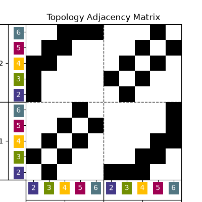
Another way to encode and visualize the geomodel topology is using an adjacency graph:

M = tp.get_adjacency_matrix(geo_model, edges, centroids)
print(M)

[[False  True False False False  True  True  True False False]
 [ True False  True False False False False  True  True False]
 [False  True False  True False False False False  True  True]
 [False False  True False  True False False False False  True]
 [False False False  True False False False False False  True]
 [ True False False False False False  True False False False]
 [ True False False False False  True False  True False False]
 [ True  True False False False False  True False  True False]
 [False  True  True False False False False  True False  True]
 [False False  True  True  True False False False  True False]]

tp.plot_adjacency_matrix(geo_model, M)

Look-up tables

The topology asset provides several look-up tables to work with the unique geobody topology id’s.

Mapping node id’s back to lithology / surface id’s:

lith_lot = tp.get_lot_node_to_lith_id(geo_model, centroids)
lith_lot

{np.int64(1): np.int64(2), np.int64(2): np.int64(3), np.int64(3): np.int64(4), np.int64(4): np.int64(5), np.int64(5): np.int64(6), np.int64(6): np.int64(2), np.int64(7): np.int64(3), np.int64(8): np.int64(4), np.int64(9): np.int64(5), np.int64(10): np.int64(6)}

Figuring out which nodes are in which fault block:

fault_lot = tp.get_lot_node_to_fault_block(geo_model, centroids)
fault_lot

{np.int64(1): np.int64(0), np.int64(2): np.int64(0), np.int64(3): np.int64(0), np.int64(4): np.int64(0), np.int64(5): np.int64(0), np.int64(6): np.int64(1), np.int64(7): np.int64(1), np.int64(8): np.int64(1), np.int64(9): np.int64(1), np.int64(10): np.int64(1)}

We can also easily map the lithology id to the corresponding topology id’s:

tp.get_lot_lith_to_node_id(lith_lot)

{np.int64(2): [np.int64(1), np.int64(6)], np.int64(3): [np.int64(2), np.int64(7)], np.int64(4): [np.int64(3), np.int64(8)], np.int64(5): [np.int64(4), np.int64(9)], np.int64(6): [np.int64(5), np.int64(10)]}

Detailed node labeling

sphinx_gallery_thumbnail_number = 4

dedges, dcentroids = tp.get_detailed_labels(geo_model, edges, centroids)

plot_2d = gpv.plot_2d(geo_model, cell_number=[5], show=False)
gpv.plot_topology(
    regular_grid=geo_model.grid.regular_grid,
    edges=dedges,
    centroids=dcentroids,
    ax=plot_2d.axes[0]
)

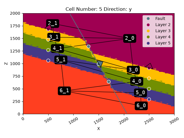
dedges

{('6_0', '6_1'), ('4_0', '5_0'), ('2_0', '3_0'), ('4_0', '5_1'), ('4_0', '6_1'), ('2_1', '3_1'), ('3_0', '4_1'), ('5_0', '6_0'), ('3_0', '5_1'), ('3_0', '4_0'), ('2_0', '3_1'), ('4_1', '5_1'), ('3_1', '4_1'), ('2_0', '2_1'), ('5_1', '6_1'), ('5_0', '6_1'), ('2_0', '4_1')}

dcentroids

{'2_0': array([35.27893175,  4.5       , 50.19485658]), '3_0': array([36.46666667,  4.5       , 29.14444444]), '4_0': array([37.59756098,  4.5       , 21.62195122]), '5_0': array([38.84563758,  4.5       , 14.00671141]), '6_0': array([39.09550562,  4.5       ,  5.37640449]), '2_1': array([ 9.79081633,  4.5       , 60.10204082]), '3_1': array([10.17687075,  4.5       , 51.02721088]), '4_1': array([11.37804878,  4.5       , 43.47560976]), '5_1': array([12.51098901,  4.5       , 35.90659341]), '6_1': array([13.659857  ,  4.5       , 15.34320735])}

Checking adjacency

So let’s say we want to check if the purple layer (id 5) is connected across the fault to the yellow layer (id 3). For this we can make easy use of the detailed labeling and the check_adjacency function:

tp.check_adjacency(dedges, "5_1", "3_0")

True

We can also check all geobodies that are adjacent to the purple layer (id 5) on the left side of the fault (fault id 1):

tp.get_adjacencies(dedges, "5_1")

{'6_1', '4_1', '4_0', '3_0'}