2D Visualization: Sections and Custom Plots

A tour of gempy_viewer’s 2D plotting options

This tutorial builds a simple faulted model with topography and two custom sections, then goes through the main plot_2d options: named sections, orthogonal cuts, the geological-map view, scalar fields, and mixing different content per panel in one figure. The last part covers retrieving the returned matplotlib figure and axes to combine several plots into a custom figure, or draw custom data (e.g. a borehole) on top of a section.

import numpy as np
import matplotlib.pyplot as plt

import gempy as gp
import gempy_viewer as gpv

np.random.seed(1234)

Model setup

The model below is the same simple fault model used throughout these tutorials: two fault blocks, each with the same four-layer stratigraphy.

data_path = 'https://raw.githubusercontent.com/cgre-aachen/gempy_data/master/'

geo_model = gp.create_geomodel(
    project_name='tutorial_2d_visualization',
    extent=[0, 2000, 0, 2000, 0, 750],
    resolution=[100, 100, 40],
    refinement=4,
    importer_helper=gp.data.ImporterHelper(
        path_to_orientations=data_path + "/data/input_data/getting_started/simple_fault_model_orientations.csv",
        path_to_surface_points=data_path + "/data/input_data/getting_started/simple_fault_model_points.csv",
        hash_surface_points="4cdd54cd510cf345a583610585f2206a2936a05faaae05595b61febfc0191563",
        hash_orientations="7ba1de060fc8df668d411d0207a326bc94a6cdca9f5fe2ed511fd4db6b3f3526"
    )
)

gp.map_stack_to_surfaces(
    gempy_model=geo_model,
    mapping_object={
        "Fault_Series": 'Main_Fault',
        "Strat_Series": ('Sandstone_2', 'Siltstone', 'Shale', 'Sandstone_1')
    }
)

gp.set_is_fault(geo_model, ["Fault_Series"])

Surface points hash:  4cdd54cd510cf345a583610585f2206a2936a05faaae05595b61febfc0191563
Orientations hash:  7ba1de060fc8df668d411d0207a326bc94a6cdca9f5fe2ed511fd4db6b3f3526

Structural Groups:	StructuralGroup: Name: Fault_Series Structural Relation: StackRelationType.FAULT Elements: StructuralElement: Name: Main_Fault StructuralGroup: Name: Strat_Series Structural Relation: StackRelationType.ERODE Elements: StructuralElement: Name: Sandstone_2 StructuralElement: Name: Siltstone StructuralElement: Name: Shale StructuralElement: Name: Sandstone_1
Fault Relations:	Fault_Seri... Strat_Seri... Fault_Series Strat_Series
	True False

Adding a random topography

set_topography_from_random generates a synthetic fractal topography over the model’s extent, which is useful for demos and tests when no real elevation data is available. It adds a topography grid to the model, which compute_model will later evaluate alongside the regular grid.

gp.set_topography_from_random(
    grid=geo_model.grid,
    fractal_dimension=1.2,
    d_z=np.array([300, 750]),
    topography_resolution=np.array([50, 50])
)

Active grids: GridTypes.DENSE|TOPOGRAPHY|NONE

Topography(_regular_grid=RegularGrid(resolution=array([100, 100,  40]), extent=array([   0., 2000.,    0., 2000.,    0.,  750.]), values=array([[  10.   ,   10.   ,    9.375],
       [  10.   ,   10.   ,   28.125],
       [  10.   ,   10.   ,   46.875],
       ...,
       [1990.   , 1990.   ,  703.125],
       [1990.   , 1990.   ,  721.875],
       [1990.   , 1990.   ,  740.625]], shape=(400000, 3)), mask_topo=array([], shape=(0, 3), dtype=bool), _transform=None, _base_resolution=array([2, 2, 2])), values_2d=array([[[   0.        ,    0.        ,  525.81364595],
        [   0.        ,   40.81632653,  534.4311714 ],
        [   0.        ,   81.63265306,  545.21138351],
        ...,
        [   0.        , 1918.36734694,  493.45417828],
        [   0.        , 1959.18367347,  505.51902125],
        [   0.        , 2000.        ,  516.62320964]],

       [[  40.81632653,    0.        ,  520.02419799],
        [  40.81632653,   40.81632653,  529.19849936],
        [  40.81632653,   81.63265306,  540.73889549],
        ...,
        [  40.81632653, 1918.36734694,  485.70563878],
        [  40.81632653, 1959.18367347,  498.13591443],
        [  40.81632653, 2000.        ,  509.94870633]],

       [[  81.63265306,    0.        ,  512.29034438],
        [  81.63265306,   40.81632653,  522.38242549],
        [  81.63265306,   81.63265306,  533.74749759],
        ...,
        [  81.63265306, 1918.36734694,  475.96047534],
        [  81.63265306, 1959.18367347,  488.33556325],
        [  81.63265306, 2000.        ,  500.75092545]],

       ...,

       [[1918.36734694,    0.        ,  536.8572301 ],
        [1918.36734694,   40.81632653,  549.32197157],
        [1918.36734694,   81.63265306,  561.72341993],
        ...,
        [1918.36734694, 1918.36734694,  503.24054915],
        [1918.36734694, 1959.18367347,  513.73925164],
        [1918.36734694, 2000.        ,  525.47837607]],

       [[1959.18367347,    0.        ,  534.68908826],
        [1959.18367347,   40.81632653,  545.65518713],
        [1959.18367347,   81.63265306,  558.27313536],
        ...,
        [1959.18367347, 1918.36734694,  501.0502999 ],
        [1959.18367347, 1959.18367347,  512.95973605],
        [1959.18367347, 2000.        ,  524.20361683]],

       [[2000.        ,    0.        ,  530.78028142],
        [2000.        ,   40.81632653,  540.15206274],
        [2000.        ,   81.63265306,  551.79148373],
        ...,
        [2000.        , 1918.36734694,  498.47649577],
        [2000.        , 1959.18367347,  510.05476038],
        [2000.        , 2000.        ,  521.16890329]]], shape=(50, 50, 3)), source=None, values=array([[   0.        ,    0.        ,  525.81364595],
       [   0.        ,   40.81632653,  534.4311714 ],
       [   0.        ,   81.63265306,  545.21138351],
       ...,
       [2000.        , 1918.36734694,  498.47649577],
       [2000.        , 1959.18367347,  510.05476038],
       [2000.        , 2000.        ,  521.16890329]], shape=(2500, 3)), resolution=(50, 50), raster_shape=())

Custom sections

A named section is a vertical cut through the model defined by two horizontal endpoints and a resolution: {'name': (start_xy, stop_xy, [n_u, n_z])}. Unlike an orthogonal cut – a single X, Y, or Z slice through the regular grid, always axis-aligned – a section can run at any angle and follow any path across the model, which makes it the way to reproduce a real geological cross-section.

Custom sections add a new grid type (SECTIONS) to the model’s grid, alongside the regular grid and topography – they aren’t something added to a plot afterwards. gempy only interpolates values on grids that are active at the time compute_model runs, so set_section_grid has to be called before computing – calling it afterwards would leave the section with no computed values to plot.

gp.set_section_grid(
    grid=geo_model.grid,
    section_dict={
        'section1': ([0, 0], [2000, 2000], [100, 80]),
        'section2': ([800, 0], [800, 2000], [150, 100])
    }
)

Active grids: GridTypes.DENSE|TOPOGRAPHY|SECTIONS|NONE

	start	stop	resolution	dist
section1	(0.0, 0.0)	(2000.0, 2000.0)	(100, 80)	2828.427125
section2	(800.0, 0.0)	(800.0, 2000.0)	(150, 100)	2000.000000

Active grids

geo_model.grid.active_grids lists which of the model’s grids will actually be evaluated on the next compute_model call. Having added a topography grid and two named sections on top of the default dense (regular) grid, all three now show up here:

geo_model.grid.active_grids

<GridTypes.DENSE|TOPOGRAPHY|SECTIONS|NONE: 1050>

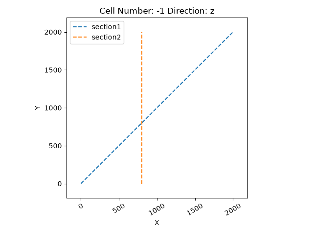
Section traces

plot_section_traces draws a map-view (top-down) plot showing where each named section actually cuts through the model – a quick way to check the sections are positioned as intended before computing:

gpv.plot_section_traces(geo_model)

<function plot_section_traces at 0x7f3efa82a980>

Computing the model

With the topography and section grids registered above, compute_model interpolates values across the regular grid and both of them in one call:

gp.compute_model(geo_model)

Setting Backend To: AvailableBackends.PYTORCH
GPU enabled. Using device: cuda
GPU device count: 1
Current GPU device: 0
Chunking done: 9 chunks
Chunking done: 50 chunks

Solutions: 4 Octree Levels, 5 DualContouringMeshes

Plotting a single section

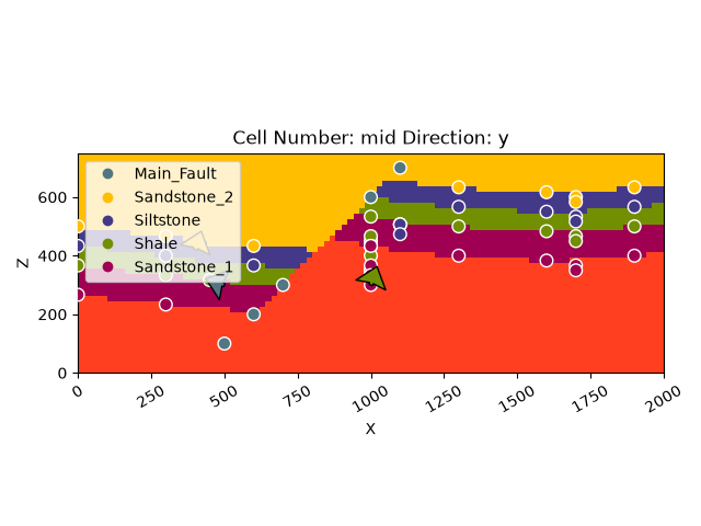
plot_2d can plot an orthogonal cut through the model: a single X, Y, or Z slice through the regular grid. Pass a cardinal direction and where along it to cut – either cell_number (an integer index into the grid’s resolution) or the string 'mid' for the middle of the model:

gpv.plot_2d(geo_model, direction=['y'], cell_number=['mid'], show_boundaries=False)

<gempy_viewer.modules.plot_2d.visualization_2d.Plot2D object at 0x7f3e54735650>

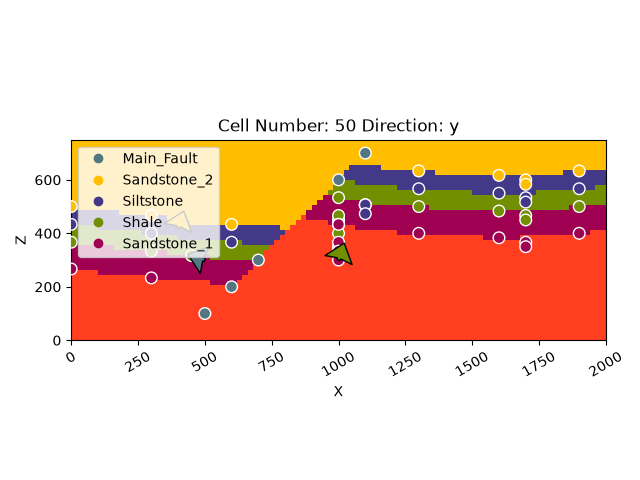
position is usually more convenient than cell_number: it takes a real-world coordinate instead of a raw grid index, which gets awkward to reason about once refinement – rather than an explicit resolution – determines the grid’s actual resolution. The plot below cuts at the same place as cell_number='mid' above (Y = 1000, the midpoint of this model’s 0-2000 extent), specified directly instead:

gpv.plot_2d(geo_model, direction=['y'], position=[1000], show_boundaries=False)

<gempy_viewer.modules.plot_2d.visualization_2d.Plot2D object at 0x7f3eea7fdbd0>

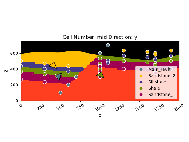
Passing show_topography=True overlays the section with its topography: the area above the actual ground surface is masked out in black, instead of showing lithology that doesn’t really exist there. This works the same way for any direction, including a horizontal ('z') cut, where it masks based on the full topography surface rather than a single profile line:

gpv.plot_2d(geo_model, direction=['y'], cell_number=['mid'], show_topography=True, show_boundaries=False)

<gempy_viewer.modules.plot_2d.visualization_2d.Plot2D object at 0x7f3eea19f3d0>

Scalar field

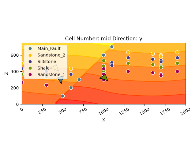
gempy solves a separate implicit scalar field per structural series – not a single field for the whole model – so series_n selects which one to plot, 0-indexed in the order the series were passed to map_stack_to_surfaces. This model has two: series 0 is Fault_Series (just the fault surface, a fairly plain field on its own) and series 1 is Strat_Series (the four stratigraphic layers), which is the more interesting one to look at since it visibly folds across the fault. Set show_scalar=True to plot a series’ scalar field, and show_lith=False to drop the lithology block underneath it so only the scalar field itself shows:

gpv.plot_2d(
    geo_model,
    direction=['y'],
    cell_number=['mid'],
    show_scalar=True,
    series_n=1,
    show_boundaries=False,
    show_lith=False
)

<gempy_viewer.modules.plot_2d.visualization_2d.Plot2D object at 0x7f3eea219250>

Contact lines only

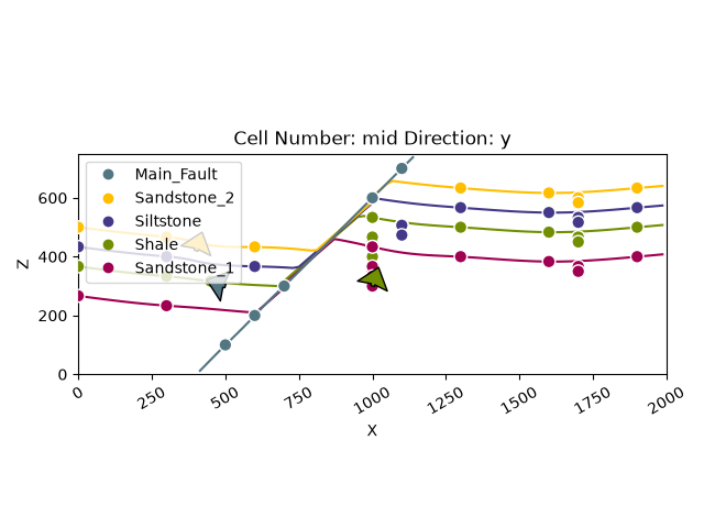
Set show_lith=False and show_boundaries=True to plot just the surface-contact isolines of the same section – the outlines where one lithology ends and the next begins – without the lithology fill:

gpv.plot_2d(geo_model, direction=['y'], cell_number=['mid'], show_lith=False, show_boundaries=True)

<gempy_viewer.modules.plot_2d.visualization_2d.Plot2D object at 0x7f3eea19f3d0>

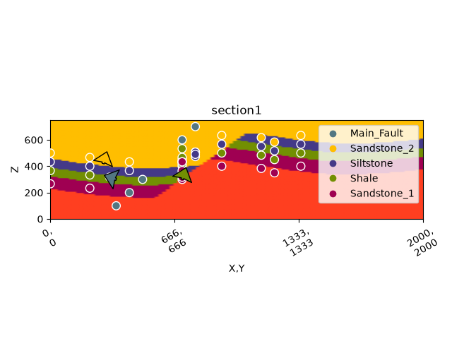
Custom sections and topography

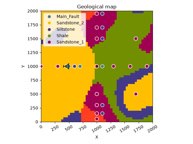
Named sections and the special section name 'topography' (a geological-map view) work exactly the same way as an orthogonal cut – the same show_lith/show_scalar/show_boundaries options all apply, just addressed via section_names instead of direction + cell_number/position:

gpv.plot_2d(geo_model, section_names=['section1'], show_boundaries=False)

<gempy_viewer.modules.plot_2d.visualization_2d.Plot2D object at 0x7f3eea1a6bd0>

gpv.plot_2d(geo_model, section_names=['topography'], show_boundaries=False)

<gempy_viewer.modules.plot_2d.visualization_2d.Plot2D object at 0x7f3eea22df50>

Combining multiple plots in one figure

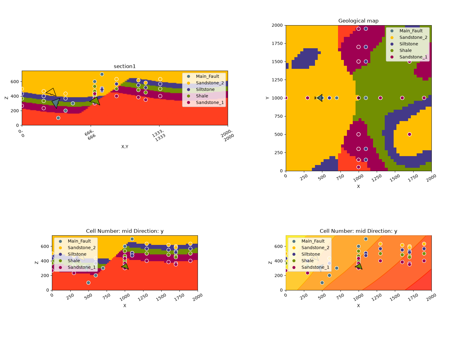
Passing several section_names and/or directions in one call builds a single figure with a subplot grid automatically, and every show_* flag also accepts a list, one entry per axis – so one figure can show all of the above side by side. Here: a named section, the geological map, a plain orthogonal section, and that same cut as a scalar field:

gpv.plot_2d(
    geo_model,
    section_names=['section1', 'topography'],
    direction=['y', 'y'],
    cell_number=['mid', 'mid'],
    show_lith=[True, True, True, False],
    show_boundaries=[False, False, False, False],
    show_scalar=[False, False, False, True]
)

<gempy_viewer.modules.plot_2d.visualization_2d.Plot2D object at 0x7f3e459c0950>

Vertical exaggeration

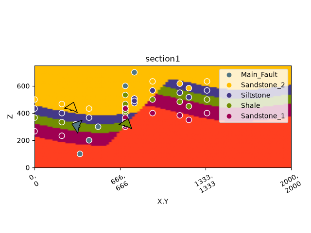
ve rescales the vertical axis of a plot and is a thin wrapper around matplotlib’s ax.set_aspect:

gpv.plot_2d(geo_model, section_names=['section1'], ve=1.5, show_boundaries=False)

<gempy_viewer.modules.plot_2d.visualization_2d.Plot2D object at 0x7f3eea1fa550>

Overlaying custom data: boreholes on a section

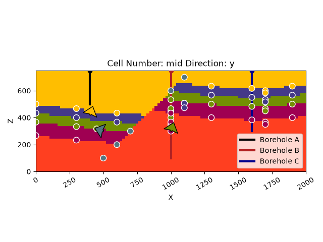
Orthogonal cuts plot directly in world X/Y/Z coordinates, so overlaying a borehole there is a plain ax.plot call. Named sections are different: their horizontal axis is distance along the section line, not world coordinates, so a world point has to be projected onto it first.

For the orthogonal case, no coordinate transform is needed – each borehole’s world X position is plotted directly against depth. All three start at the model’s top (extent[5]) and reach different depths:

z_top = geo_model.grid.regular_grid.extent[5]
boreholes_ortho = [
    {'name': 'Borehole A', 'x': 400, 'z_bottom': 500, 'color': 'black'},
    {'name': 'Borehole B', 'x': 1000, 'z_bottom': 100, 'color': 'firebrick'},
    {'name': 'Borehole C', 'x': 1600, 'z_bottom': 300, 'color': 'darkblue'},
]

p_ortho = gpv.plot_2d(geo_model, direction=['y'], cell_number=['mid'], show_boundaries=False, show=False)
ax_ortho = p_ortho.axes[0]
for bh in boreholes_ortho:
    ax_ortho.plot([bh['x'], bh['x']], [bh['z_bottom'], z_top], color=bh['color'], linewidth=3, label=bh['name'])
    ax_ortho.scatter([bh['x']], [z_top], color=bh['color'], zorder=10)
ax_ortho.legend()

plt.show()

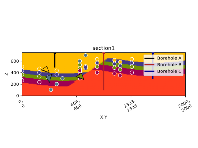
For a named section, each borehole’s (x, y) collar first needs to be projected onto the section’s start -> stop line to get its position along the section axis; depth (z) still plots directly. start and stop are stored per section in grid.sections.df:

section_name = 'section1'
sections_df = geo_model.grid.sections.df
start = np.array(sections_df.loc[section_name, 'start'], dtype=float)
stop = np.array(sections_df.loc[section_name, 'stop'], dtype=float)
u_hat = (stop - start) / np.linalg.norm(stop - start)


def project_onto_section(point_xy, start, u_hat):
    return np.dot(np.asarray(point_xy, dtype=float) - start, u_hat)


boreholes_section = [
    {'name': 'Borehole A', 'xy': [400, 400], 'z_bottom': 500, 'color': 'black'},
    {'name': 'Borehole B', 'xy': [1000, 1000], 'z_bottom': 100, 'color': 'firebrick'},
    {'name': 'Borehole C', 'xy': [1600, 1600], 'z_bottom': 300, 'color': 'darkblue'},
]

p_section = gpv.plot_2d(geo_model, section_names=[section_name], show_boundaries=False, show=False)
ax_section = p_section.axes[0]
for bh in boreholes_section:
    u = project_onto_section(bh['xy'], start, u_hat)
    ax_section.plot([u, u], [bh['z_bottom'], z_top], color=bh['color'], linewidth=3, label=bh['name'])
    ax_section.scatter([u], [z_top], color=bh['color'], zorder=10)
ax_section.legend()

plt.show()

# sphinx_gallery_thumbnail_number = -1