Note
Go to the end to download the full example code.
Video Tutorial “code-along”: Onlap relations
This tutorial demonstrates step-by-step how to incorporate onlap relations to our geological models created with gempy. It follows the Video tutorial series available on the [gempy YouTube channel](https://www.youtube.com/@GemPy3D). Please follow the first and second part of the tutorials to learn the basics of modeling with gempy before diving into this tutorial.
Video tutorial 11: Basic onlap scenario
# Required imports
import gempy as gp
import gempy_viewer as gpv
import numpy as np
# Path to input data
data_path = "https://raw.githubusercontent.com/cgre-aachen/gempy_data/master/"
path_to_data = data_path + "/data/input_data/video_tutorials_v3/"
# Create instance of geomodel
geo_model_onlap = gp.create_geomodel(
    project_name = 'tutorial_model_onlap_1',
    extent=[0,2000,0,1000,0,1000],
    resolution=[100,50,50],
    importer_helper=gp.data.ImporterHelper(
        path_to_orientations=path_to_data+"tutorial_model_onlap_1_orientations.csv",
        path_to_surface_points=path_to_data+"tutorial_model_onlap_1_surface_points.csv"
    )
)
Surface points hash:  2de2814bb46c6cbaa69572685aff54886e4ce3e3620384a0c70e3c52b71c0bd1
Orientations hash:  059fe82183b03d9c50b4eb8249e2ea99297a704ce85138678a7d93e7d19b7b12
# Map geological series to surfaces
gp.map_stack_to_surfaces(
    gempy_model=geo_model_onlap,
    mapping_object={
        "Young_Series": ("basin_fill_2", "basin_fill_1"),
        "Old_Series": ("basin_top", "basin_bottom")
    }
)

# Alternative way of mapping geological series to surfaces
# gp.map_stack_to_surfaces(
#     gempy_model=geo_model_onlap,
#     mapping_object={
#         "Young_Series": ("basin_fill_2", "basin_fill_1"),
#         "Onlap_Series": ("basin_top"),
#         "Old_Series": ("basin_bottom")
#     }
# )
# Display a basic cross section of input data
gpv.plot_2d(geo_model_onlap, show_data=True)
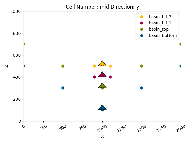
<gempy_viewer.modules.plot_2d.visualization_2d.Plot2D object at 0x7f58216baa50>
# Compute a solution for the model
gp.compute_model(geo_model_onlap)
Setting Backend To: AvailableBackends.PYTORCH
GPU requested but unavailable; falling back to CPU (GEMPY_GPU_FALLBACK=True)
Setting Backend To: AvailableBackends.PYTORCH
Chunking done: 10 chunks
Chunking done: 19 chunks
# Display the result in 2d section
gpv.plot_2d(geo_model_onlap, show_boundaries=False)
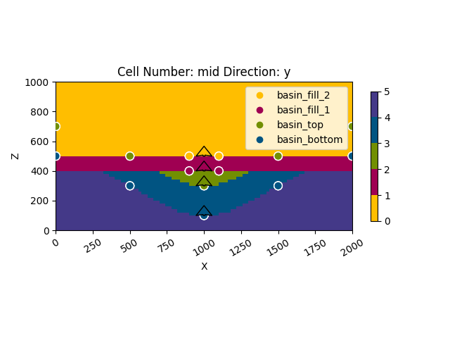
<gempy_viewer.modules.plot_2d.visualization_2d.Plot2D object at 0x7f57780539d0>
# Set the relation of the youngest group to Onlap
from gempy_engine.core.data.stack_relation_type import StackRelationType
geo_model_onlap.structural_frame.structural_groups[0].structural_relation = StackRelationType.ONLAP
# Display updated strucutral frame
geo_model_onlap.structural_frame
# Compute a solution for the model
gp.compute_model(geo_model_onlap)
Setting Backend To: AvailableBackends.PYTORCH
GPU requested but unavailable; falling back to CPU (GEMPY_GPU_FALLBACK=True)
Setting Backend To: AvailableBackends.PYTORCH
Chunking done: 10 chunks
Chunking done: 19 chunks
# Display the result in 2d section
gpv.plot_2d(geo_model_onlap, show_boundaries=False)
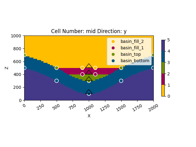
<gempy_viewer.modules.plot_2d.visualization_2d.Plot2D object at 0x7f580ed8a4d0>
Video tutorial 12: Advanced onlap - Subduction zone
# Create instance of geomodel
geo_model_subduction = gp.create_geomodel(
    project_name = 'tutorial_model_onlap_2',
    extent=[0,2000,0,1000,0,1000],
    resolution=[100,50,50],
    importer_helper=gp.data.ImporterHelper(
        path_to_orientations=path_to_data+"tutorial_model_onlap_2_orientations.csv?",
        path_to_surface_points=path_to_data+"tutorial_model_onlap_2_surface_points.csv?"
    )
)
Surface points hash:  d0999adb1b7cfca54abd040f517aeba042d7f43a69b507c69ac6ad8cd6682e13
Orientations hash:  ebada610b5a68730bf1d03323594e755fbe986cd07857ee99d8b758716e3dfaa
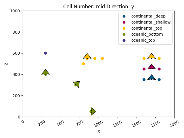
# Display a basic cross section of input data
gpv.plot_2d(geo_model_subduction)
<gempy_viewer.modules.plot_2d.visualization_2d.Plot2D object at 0x7f57781087d0>
# Map geological series to surfaces
gp.map_stack_to_surfaces(
    gempy_model=geo_model_subduction,
    mapping_object={
        "Top": ("continental_top"),
        "Continental_Series": ("continental_shallow", "continental_deep"),
        "Oceanic_Series": ("oceanic_top", "oceanic_bottom")
    }
)
# Set the realtion of the youngest and second youngest group to Onlap
geo_model_subduction.structural_frame.structural_groups[0].structural_relation = StackRelationType.ONLAP
geo_model_subduction.structural_frame.structural_groups[1].structural_relation = StackRelationType.ONLAP
# Display updated structural frame
geo_model_subduction.structural_frame
# Create a simple topography using numpy

# Define grid spacing
spacing = 20

# Generate grid
x = np.arange(geo_model_subduction.grid.regular_grid.extent[0], geo_model_subduction.grid.regular_grid.extent[1] + spacing, spacing)
y = np.arange(geo_model_subduction.grid.regular_grid.extent[2], geo_model_subduction.grid.regular_grid.extent[3] + spacing, spacing)
X, Y = np.meshgrid(x, y)

# Define elevation (z) based on x, creating a simple mountain range
Z = np.ones_like(X) * 590  # Default elevation
Z[(X >= 570) & (X < 1000)] = 590 + (200 * (X[(X >= 570) & (X < 1000)] - 600) / 400)
Z[(X >= 1000) & (X < 1300)] = 810 - (250 * (X[(X >= 1000) & (X < 1300)] - 1000) / 300)
Z[X >= 1300] = 540

# Flatten the data into (N,3) shape
topography_points = np.vstack((X.ravel(), Y.ravel(), Z.ravel())).T
# Set topography from numpy array
gp.set_topography_from_arrays(grid=geo_model_subduction.grid, xyz_vertices=topography_points)
Active grids: GridTypes.DENSE|TOPOGRAPHY|NONE

Topography(_regular_grid=RegularGrid(resolution=array([100,  50,  50]), extent=array([   0., 2000.,    0., 1000.,    0., 1000.]), values=array([[  10.,   10.,   10.],
       [  10.,   10.,   30.],
       [  10.,   10.,   50.],
       ...,
       [1990.,  990.,  950.],
       [1990.,  990.,  970.],
       [1990.,  990.,  990.]], shape=(250000, 3)), mask_topo=array([], shape=(0, 3), dtype=bool), _transform=None, _base_resolution=array([2, 2, 2])), values_2d=array([[[   0.        ,    0.        ,  590.        ],
        [   0.        ,   20.40816327,  590.        ],
        [   0.        ,   40.81632653,  590.        ],
        ...,
        [   0.        ,  959.18367347,  590.        ],
        [   0.        ,  979.59183673,  590.        ],
        [   0.        , 1000.        ,  590.        ]],

       [[  20.2020202 ,    0.        ,  590.        ],
        [  20.2020202 ,   20.40816327,  590.        ],
        [  20.2020202 ,   40.81632653,  590.        ],
        ...,
        [  20.2020202 ,  959.18367347,  590.        ],
        [  20.2020202 ,  979.59183673,  590.        ],
        [  20.2020202 , 1000.        ,  590.        ]],

       [[  40.4040404 ,    0.        ,  590.        ],
        [  40.4040404 ,   20.40816327,  590.        ],
        [  40.4040404 ,   40.81632653,  590.        ],
        ...,
        [  40.4040404 ,  959.18367347,  590.        ],
        [  40.4040404 ,  979.59183673,  590.        ],
        [  40.4040404 , 1000.        ,  590.        ]],

       ...,

       [[1959.5959596 ,    0.        ,  540.        ],
        [1959.5959596 ,   20.40816327,  540.        ],
        [1959.5959596 ,   40.81632653,  540.        ],
        ...,
        [1959.5959596 ,  959.18367347,  540.        ],
        [1959.5959596 ,  979.59183673,  540.        ],
        [1959.5959596 , 1000.        ,  540.        ]],

       [[1979.7979798 ,    0.        ,  540.        ],
        [1979.7979798 ,   20.40816327,  540.        ],
        [1979.7979798 ,   40.81632653,  540.        ],
        ...,
        [1979.7979798 ,  959.18367347,  540.        ],
        [1979.7979798 ,  979.59183673,  540.        ],
        [1979.7979798 , 1000.        ,  540.        ]],

       [[2000.        ,    0.        ,  540.        ],
        [2000.        ,   20.40816327,  540.        ],
        [2000.        ,   40.81632653,  540.        ],
        ...,
        [2000.        ,  959.18367347,  540.        ],
        [2000.        ,  979.59183673,  540.        ],
        [2000.        , 1000.        ,  540.        ]]],
      shape=(100, 50, 3)), source=None, values=array([[   0.        ,    0.        ,  590.        ],
       [   0.        ,   20.40816327,  590.        ],
       [   0.        ,   40.81632653,  590.        ],
       ...,
       [2000.        ,  959.18367347,  540.        ],
       [2000.        ,  979.59183673,  540.        ],
       [2000.        , 1000.        ,  540.        ]], shape=(5000, 3)), resolution=(100, 50), raster_shape=())
# Compute a solution for the model
gp.compute_model(geo_model_subduction)
Setting Backend To: AvailableBackends.PYTORCH
GPU requested but unavailable; falling back to CPU (GEMPY_GPU_FALLBACK=True)
Setting Backend To: AvailableBackends.PYTORCH
Chunking done: 14 chunks
Chunking done: 10 chunks
Chunking done: 12 chunks
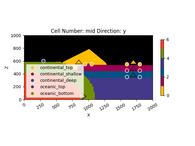
# Display the result in 2d section
gpv.plot_2d(geo_model_subduction, show_topography=True, show_boundaries=False)
<gempy_viewer.modules.plot_2d.visualization_2d.Plot2D object at 0x7f57ec7a7450>
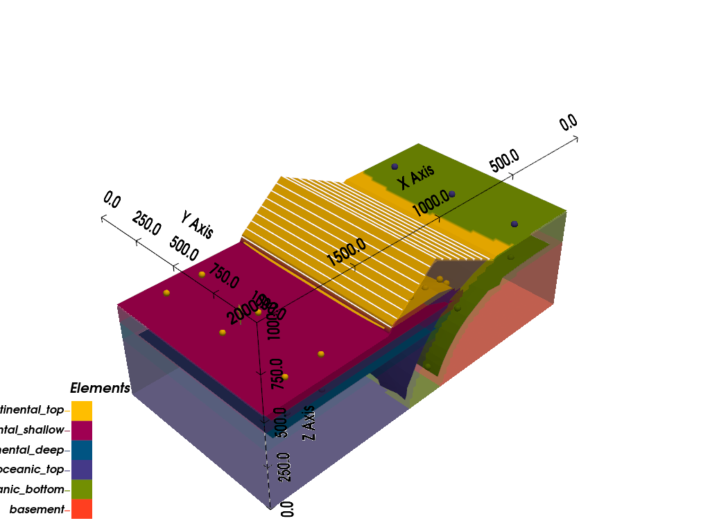
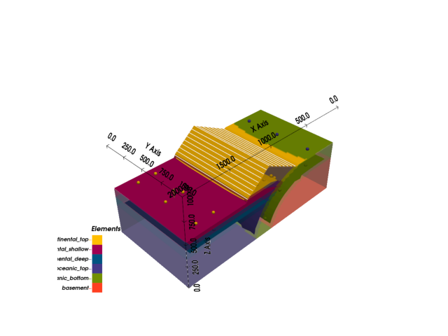
# Display 3d plot of final model
gpv.plot_3d(geo_model_subduction, show_topography=True, image=True)

# sphinx_gallery_thumbnail_number = -1
<gempy_viewer.modules.plot_3d.vista.GemPyToVista object at 0x7f578039bcb0>
Total running time of the script: (0 minutes 10.838 seconds)