Geomodeling benchmark: the “Moureze”-Model

This model is part of a geomodeling benchmaring effort. More information (and, hopefully, publication) coming.

import os

These two lines are necessary only if gempy is not installed

# Importing gempy
import gempy as gp
import gempy_viewer as gpv

# Aux imports
import numpy as np
import pandas as pd

from gempy_engine.config import AvailableBackends

Loading surface points from repository:

With pandas we can do it directly from the web and with the right args we can directly tidy the data in gempy style:

data_path = os.path.abspath('../../data/input_data/Moureze')
Moureze_points = pd.read_csv(
    filepath_or_buffer=data_path + '/Moureze_Points.csv',
    sep=';',
    names=['X', 'Y', 'Z', 'G_x', 'G_y', 'G_z', '_'],
    header=0,
)

Sections_EW = pd.read_csv(
    filepath_or_buffer=data_path + '/Sections_EW.csv',
    sep=';',
    names=['X', 'Y', 'Z', 'ID', '_'], header=1
).dropna()

Sections_NS = pd.read_csv(
    filepath_or_buffer=data_path + '/Sections_NS.csv',
    sep=';',
    names=['X', 'Y', 'Z', 'ID', '_'], header=1
).dropna()

Extracting the orientatins:

mask_surfpoints = Moureze_points['G_x'] < -9999
surface_points = Moureze_points[mask_surfpoints][::10]
orientations = Moureze_points[~mask_surfpoints][::10]

Giving an arbitrary value name to the surface

surface_points['surface'] = '0'
orientations['surface'] = '0'

surface_points.tail()

	X	Y	Z	G_x	G_y	G_z	_	surface
3370	224.00	65.34	-120.00	-99999.0	-99999.0	-99999.0	0.67	0
3386	232.00	20.00	-85.10	-99999.0	-99999.0	-99999.0	0.70	0
3396	135.94	154.31	-154.02	-99999.0	-99999.0	-99999.0	0.35	0
3411	296.00	378.00	-156.41	-99999.0	-99999.0	-99999.0	0.85	0
3424	91.96	151.81	-83.26	-99999.0	-99999.0	-99999.0	0.95	0

orientations.tail()

	X	Y	Z	G_x	G_y	G_z	_	surface
3186	139.94	207.71	-154.77	-0.03	0.07	1.00	0.05	0
3254	109.93	47.65	-135.34	0.35	-0.77	-0.54	0.94	0
3315	158.34	211.32	-147.31	0.05	0.14	0.99	0.05	0
3371	0.73	90.00	-100.00	0.76	0.53	0.38	0.17	0
3409	47.97	129.89	-132.01	-0.45	-0.85	0.27	0.02	0

Data initialization:

Suggested size of the axis-aligned modeling box:

Origin: -5 -5 -200

Maximum: 305 405 -50

Suggested resolution: 2m (grid size 156 x 206 x 76)

Only using one orientation because otherwhise it gets a mess

Number voxels

np.array([156, 206, 76]).prod()

2442336

resolution_requ = [156, 206, 76]
resolution = [77, 103, 38]
resolution_low = [45, 51, 38]


surface_points_table: gp.data.SurfacePointsTable = gp.data.SurfacePointsTable.from_arrays(
    x=surface_points['X'].values,
    y=surface_points['Y'].values,
    z=surface_points['Z'].values,
    names=surface_points['surface'].values.astype(str)
)

orientations_table: gp.data.OrientationsTable = gp.data.OrientationsTable.from_arrays(
    x=orientations['X'].values,
    y=orientations['Y'].values,
    z=orientations['Z'].values,
    G_x=orientations['G_x'].values,
    G_y=orientations['G_y'].values,
    G_z=orientations['G_z'].values,
    names=orientations['surface'].values.astype(str),
    name_id_map=surface_points_table.name_id_map  # ! Make sure that ids and names are shared
)

structural_frame: gp.data.StructuralFrame = gp.data.StructuralFrame.from_data_tables(
    surface_points=surface_points_table,
    orientations=orientations_table
)

geo_model: gp.data.GeoModel = gp.create_geomodel(
    project_name='Moureze',
    extent=[-5, 305, -5, 405, -200, -50],
    # resolution=resolution_low,
    refinement=5,
    structural_frame=structural_frame
)

Now we can see how the data looks so far:

gpv.plot_2d(geo_model, direction='y')

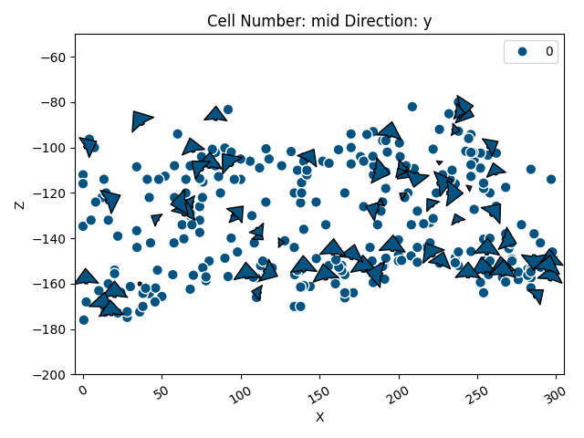
<gempy_viewer.modules.plot_2d.visualization_2d.Plot2D object at 0x7fcd8fee28f0>

The default range is always the diagonal of the extent. Since in this model data is very close we will need to reduce the range to 5-10% of that value:

geo_model.interpolation_options.kernel_options.range *= 0.2
geo_model.interpolation_options.evaluation_options.verbose = True
geo_model.interpolation_options.evaluation_options.octree_error_threshold = 1.5
geo_model.interpolation_options.evaluation_options.number_octree_levels_surface = 5

gp.compute_model(
    gempy_model=geo_model,
    engine_config=gp.data.GemPyEngineConfig(
        use_gpu=False,
        dtype='float32',
        backend=AvailableBackends.PYTORCH
    )
)

• 
• 

Setting Backend To: AvailableBackends.PYTORCH
Number of voxels marked by stats: 437 of torch.Size([512]).
 Number of voxels marked by corners : 408
Total voxels: 437
Dense Grid would be 512 voxels
Chunking done: 30 chunks
Number of voxels marked by stats: 3053 of torch.Size([3736]).
 Number of voxels marked by corners : 1993
Total voxels: 3053
Dense Grid would be 4096 voxels
Chunking done: 25 chunks
Chunking done: 197 chunks
Chunking done: 35 chunks

Solutions: 5 Octree Levels, 1 DualContouringMeshes

Time

300k voxels 3.5k points

• Nvidia 2080: 500 ms ± 1.3 ms per loop (mean ± std. dev. of 7 runs, 1 loop each), Memory 1 Gb

• CPU 14.2 s ± 82.4 ms per loop (mean ± std. dev. of 7 runs, 1 loop each), Memory: 1.3 Gb

2.4 M voxels, 3.5k points

• CPU 2min 33s ± 216 ms per loop (mean ± std. dev. of 7 runs, 1 loop each) Memory: 1.3 GB

• Nvidia 2080: 1.92 s ± 6.74 ms per loop (mean ± std. dev. of 7 runs, 1 loop each) 1 Gb

2.4 M voxels, 3.5k points 3.5 k orientations

• Nvidia 2080: 2.53 s ± 1.31 ms per loop (mean ± std. dev. of 7 runs, 1 loop each)

gpv.plot_2d(geo_model, cell_number='mid', series_n=0, show_scalar=True)

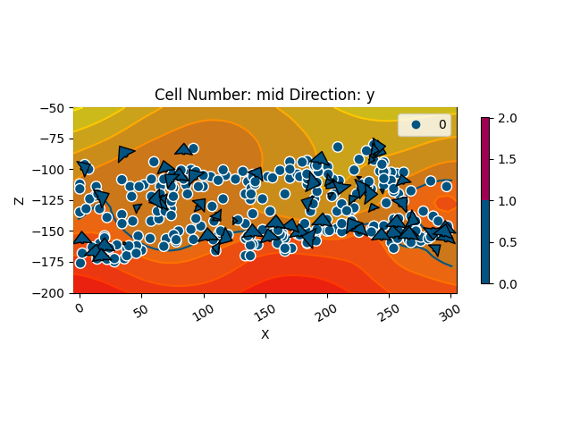
<gempy_viewer.modules.plot_2d.visualization_2d.Plot2D object at 0x7fcd8fee0280>

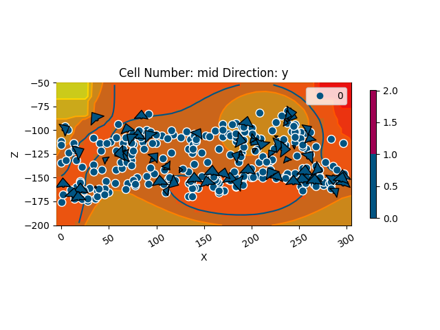
gpv.plot_2d(geo_model, cell_number='mid', show_data=True, direction='y')

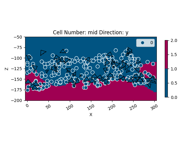
<gempy_viewer.modules.plot_2d.visualization_2d.Plot2D object at 0x7fcdce7e40a0>

sphinx_gallery_thumbnail_number = 4

gpv.plot_3d(geo_model)

<gempy_viewer.modules.plot_3d.vista.GemPyToVista object at 0x7fcd8fee0280>