Modeling step by step

This tutorial demonstrates step-by-step geological modeling using the gempy and gempy_viewer libraries. We will start by importing the necessary packages, loading input data, creating a geological model, and then visualizing the results.

Import minimal requirements We need to import the gempy library for geological modeling and gempy_viewer for visualization.

import gempy as gp
import gempy_viewer as gpv

Define the path to input data Here, we provide two ways to define the path to the input data: using a URL or a local path. Uncomment the first two lines if you want to use the online data source.

# data_path = 'https://raw.githubusercontent.com/cgre-aachen/gempy_data/master/'
# path_to_data = data_path + "/data/input_data/jan_models/"

# For this tutorial, we will use the local path:
data_path = '../../'
path_to_data = data_path + "/data/input_data/jan_models/"

Create a GeoModel instance We create a GeoModel instance with a specified project name and extent. The ImporterHelper class is used to specify the paths to the orientation and surface points data.

geo_model = gp.create_geomodel(
    project_name='tutorial_model',
    extent=[0, 2500, 0, 1000, 0, 1110],
    refinement=4,
    importer_helper=gp.data.ImporterHelper(
        path_to_orientations=path_to_data + "tutorial_model_orientations.csv",
        path_to_surface_points=path_to_data + "tutorial_model_surface_points.csv"
    )
)

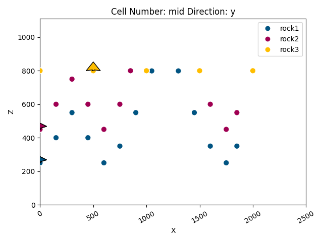
Displaying simple data cross section We use the gempy_viewer to visualize the initial cross-section of our geological model.

gpv.plot_2d(geo_model)

<gempy_viewer.modules.plot_2d.visualization_2d.Plot2D object at 0x7f87cc6df8b0>

Map geological series to surfaces Here, we map the geological series to specific surfaces. This step is crucial for defining the stratigraphic relationships in our model.

gp.map_stack_to_surfaces(
    gempy_model=geo_model,
    mapping_object={
            "Strat_Series1": ('rock3'),
            "Strat_Series2": ('rock2', 'rock1'),
    }
)

Structural Groups:	StructuralGroup: Name: Strat_Series1 Structural Relation: StackRelationType.ERODE Elements: StructuralElement: Name: rock3 StructuralGroup: Name: Strat_Series2 Structural Relation: StackRelationType.ERODE Elements: StructuralElement: Name: rock2 StructuralElement: Name: rock1
Fault Relations:	Strat_Seri... Strat_Seri... Strat_Series1 Strat_Series2
	True False

Update transformation and interpolation options We update the model with anisotropy settings and specify various interpolation options to refine the model’s accuracy.

geo_model.update_transform(auto_anisotropy=gp.data.GlobalAnisotropy.CUBE)

interpolation_options: gp.data.InterpolationOptions = geo_model.interpolation_options

interpolation_options.kernel_options.range = 1.7
interpolation_options.evaluation_options.number_octree_levels_surface = 4
interpolation_options.evaluation_options.compute_scalar_gradient = False
interpolation_options.evaluation_options.curvature_threshold = 1
interpolation_options.evaluation_options.min_octree_level = 1

interpolation_options.evaluation_options.verbose = True

Compute the geological model We use the specified backend (in this case, PyTorch) to compute the model.

gp.compute_model(
    gempy_model=geo_model,
    engine_config=gp.data.GemPyEngineConfig(
        backend=gp.data.AvailableBackends.numpy,
        dtype="float64"
    )
)

• 
• 
• 
• 

Setting Backend To: AvailableBackends.numpy
Number of voxels marked by stats: 16 of (64,).
 Number of voxels marked by corners : 40
Total voxels: 16
Dense Grid would be 64 voxels
Number of voxels marked by stats: 40 of (64,).
 Number of voxels marked by corners : 40
Total voxels: 44
Dense Grid would be 64 voxels
Number of voxels marked by stats: 128 of (384,).
 Number of voxels marked by corners : 232
Total voxels: 128
Dense Grid would be 512 voxels
Number of voxels marked by stats: 216 of (384,).
 Number of voxels marked by corners : 232
Total voxels: 240
Dense Grid would be 512 voxels

Solutions: 4 Octree Levels, 3 DualContouringMeshes

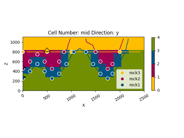
Visualize the model: 2D cross-section without scalar field After computing the model, we visualize it again in 2D without the scalar field.

gpv.plot_2d(geo_model, show_scalar=False, series_n=1)

<gempy_viewer.modules.plot_2d.visualization_2d.Plot2D object at 0x7f87dbafbb80>

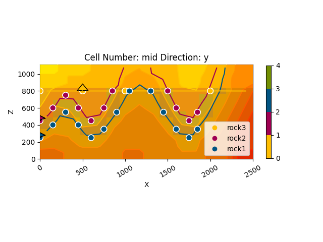
Visualize the model: 2D cross-section with scalar field In this cell, we visualize the 2D cross-section with the scalar field enabled. %%

gpv.plot_2d(geo_model, show_scalar=True, series_n=1)

<gempy_viewer.modules.plot_2d.visualization_2d.Plot2D object at 0x7f87cc542860>

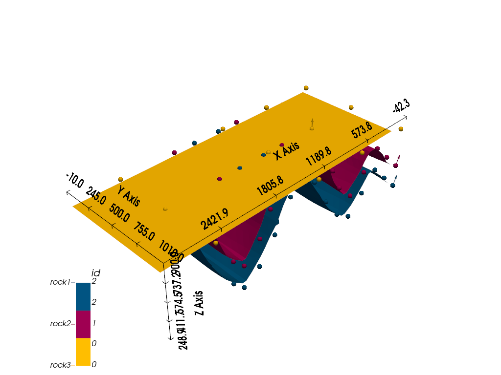
Visualize the model in 3D Finally, we create a 3D visualization of the geological model without lithological coloring and image.

gpv.plot_3d(geo_model, show_lith=False, image=False)
# sphinx_gallery_thumbnail_number = -1

<gempy_viewer.modules.plot_3d.vista.GemPyToVista object at 0x7f87cc7ce6b0>

### Coming up next Additional: Manually adding data (optional) Here is an example of how you can manually add surface points to the model. Uncomment and modify the code as needed.

'''
gp.add_surface_points(
    geo_model=geo_model,
    x=[458, 612],
    y=[0, 0],
    z=[-107, -14],
    elements_names=['surface1', 'surface1']
)
'''

"\ngp.add_surface_points(\n    geo_model=geo_model,\n    x=[458, 612],\n    y=[0, 0],\n    z=[-107, -14],\n    elements_names=['surface1', 'surface1']\n)\n"

Displaying data cross section (optional) You can re-plot the 2D cross-section if needed. gpv.plot_2d(geo_model) %%