3.1: Simple example of kriging in gempy

In this notebook it will be shown how to create a kriged or simulated field in a simple geological model in gempy. We start by creating a simple model with three horizontally layered units, as shown in the gempy examples.

Importing GemPy

import gempy as gp
import gempy_viewer as gpv

# Importing auxiliary libraries
import numpy as np
import matplotlib.pyplot as plt
import os

# new for this
from gempy_plugins.kriging import kriging

np.random.seed(5555)

Creating the model by importing the input data and displaying it:

data_path = os.path.abspath('../../')

geo_data: gp.data.GeoModel = gp.create_geomodel(
    project_name='kriging',
    extent=[0, 1000, 0, 50, 0, 1000],
    resolution=[50, 10, 50],
    refinement=1,
    importer_helper=gp.data.ImporterHelper(
        path_to_orientations=data_path + "/data/input_data/jan_models/model1_orientations.csv",
        path_to_surface_points=data_path + "/data/input_data/jan_models/model1_surface_points.csv",
    )
)

Setting and ordering the units and series:

gp.map_stack_to_surfaces(
    gempy_model=geo_data,
    mapping_object={
        "Strat_Series": ('rock2', 'rock1'),
        "Basement_Series": ('basement')
    }
)

Could not find element 'basement' in any group.

Structural Groups:	StructuralGroup: Name: Strat_Series Structural Relation: StackRelationType.ERODE Elements: StructuralElement: Name: rock2 StructuralElement: Name: rock1
Fault Relations:	Strat_Seri... Strat_Series
	True False

Calculating the model:

no mesh computed as basically 2D model

sol = gp.compute_model(geo_data)

Setting Backend To: AvailableBackends.numpy
/home/leguark/gempy_engine/gempy_engine/modules/dual_contouring/dual_contouring_interface.py:38: RuntimeWarning: divide by zero encountered in divide
  weight_x = ((scalar_at_sp - scalar_8[:, :, 4:]) / scalar_dx).reshape(-1, 4, 1)
/home/leguark/gempy_engine/gempy_engine/modules/dual_contouring/dual_contouring_interface.py:39: RuntimeWarning: divide by zero encountered in divide
  weight_y = ((scalar_at_sp - scalar_8[:, :, [2, 3, 6, 7]]) / scalar_d_y).reshape(-1, 4, 1)
/home/leguark/gempy_engine/gempy_engine/modules/dual_contouring/dual_contouring_interface.py:48: RuntimeWarning: invalid value encountered in multiply
  intersect_dx = d_x[:, :, :] * weight_x[:, :, :]
/home/leguark/gempy_engine/gempy_engine/modules/dual_contouring/dual_contouring_interface.py:49: RuntimeWarning: invalid value encountered in multiply
  intersect_dy = d_y[:, :, :] * weight_y[:, :, :]

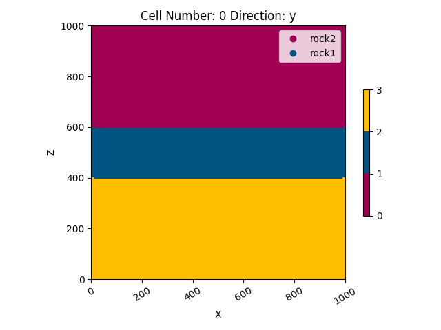
So here is the very simple, basically 2D model that we created:

gpv.plot_2d(geo_data, cell_number=0, show_data=False)

<gempy_viewer.modules.plot_2d.visualization_2d.Plot2D object at 0x7f490cb745e0>

1) Creating domain

Let us assume we have a couple of measurements in a domain of interest within our model. In our case the unit of interest is the central rock layer (rock1). In the kriging module we can define the domain by handing over a number of surfaces by id - in this case the id of rock1 is 2. In addition we define four input data points in cond_data, each defined by x,y,z coordinate and a measurement value.

conditioning data (data measured at locations)

cond_data = np.array([[100, .5, 500, 2], [900, .5, 500, 1],
                      [500, .5, 550, 1], [300, .5, 400, 5]])

creating a domain object from the gempy solution, a defined domain conditioning data

domain = kriging.Domain(
    model_solutions=sol,
    transform=geo_data.transform,
    domain=[2],
    data=cond_data
)

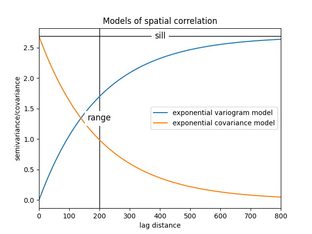
2) Creating a variogram model

variogram_model = kriging.VariogramModel(
    theoretical_model='exponential',
    range_=200,
    sill=np.var(cond_data[:, 3])
)

variogram_model.plot(type_='both', show_parameters=True)
plt.show()

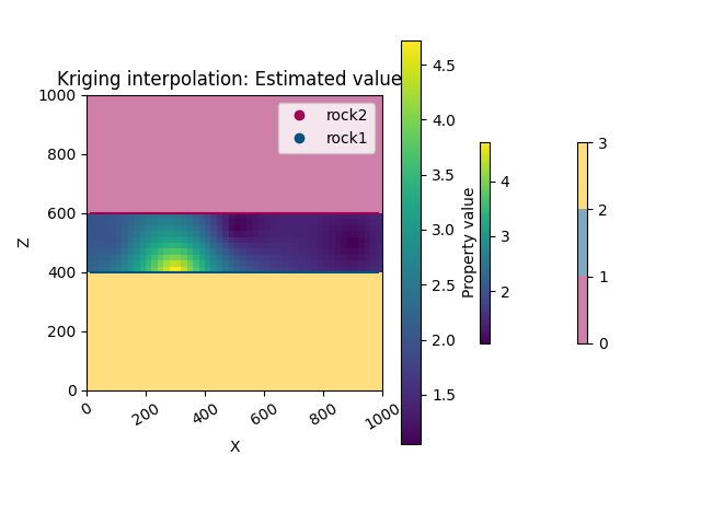
3) Kriging interpolation

In the following we define an object called kriging_model and set all input parameters. Finally we generate the kriged field.

kriging_solution = kriging.create_kriged_field(domain, variogram_model)

The result of our calculation is saved in the following dataframe, containing an estimated value and the kriging variance for each point in the grid:

kriging_solution.results_df.head()

	X	Y	Z	estimated value	estimation variance
0	10.0016	2.5016	410.0016	2.241542	2.103698
1	10.0016	2.5016	430.0016	2.193555	1.979810
2	10.0016	2.5016	450.0016	2.144345	1.865440
3	10.0016	2.5016	470.0016	2.097883	1.774970
4	10.0016	2.5016	490.0016	2.058535	1.724997

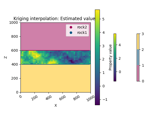
It is also possible to plot the results in cross section similar to the way gempy models are plotted.

from gempy_viewer.modules.plot_2d.visualization_2d import Plot2D

plot_2d: Plot2D = gpv.plot_2d(
    model=geo_data,
    cell_number=0,
    show_data=False,
    show=False,
    kwargs_lithology={ 'alpha': 0.5 }
)
kriging.plot_kriging_results(
    geo_data=geo_data,
    kriging_solution=kriging_solution,
    plot_2d=plot_2d,
    title='Kriging interpolation: Estimated values',
    result_column=['estimated value']
)

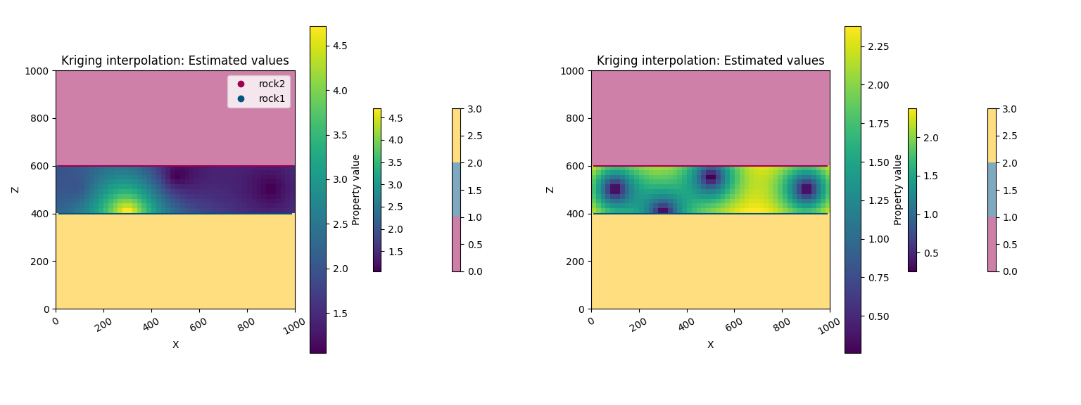
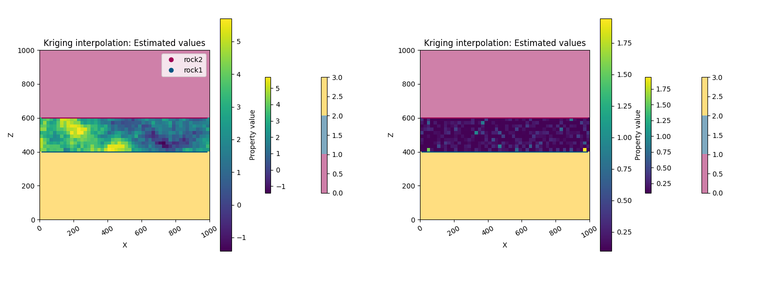
plot_2d_both = gpv.plot_2d(
    model=geo_data,
    cell_number=[0, 0],
    show_data=False,
    show=False,
    kwargs_lithology={ 'alpha': 0.5 }
)

kriging.plot_kriging_results(
    geo_data=geo_data,
    kriging_solution=kriging_solution,
    plot_2d=plot_2d_both,
    title='Kriging interpolation: Estimated values',
    result_column=['estimated value', 'estimation variance']
)

4) Simulated field

Based on the same objects (domain and varigoram model) also a simulated field (stationary Gaussian Field) can be generated. A Sequential Gaussian Simulation approach is applied in this module:

solution_sim = kriging.create_gaussian_field(domain, variogram_model)

solution_sim.results_df.head()

	X	Y	Z	estimated value	estimation variance
1774	10.0016	2.5016	410.0016	4.420467	0.122209
4701	10.0016	2.5016	430.0016	4.893653	0.108040
3463	10.0016	2.5016	450.0016	4.874381	0.177325
3227	10.0016	2.5016	470.0016	4.983143	0.220953
4528	10.0016	2.5016	490.0016	3.747620	0.108041

solution_sim.results_df['estimated value']

1774    4.420467
4701    4.893653
3463    4.874381
3227    4.983143
4528    3.747620
          ...
1712    3.540901
390     3.863402
1039    4.134937
3379    3.144726
4090    2.446597
Name: estimated value, Length: 5000, dtype: float64

plot_2d: Plot2D = gpv.plot_2d(
    model=geo_data,
    cell_number=0,
    show_data=False,
    show=False,
    kwargs_lithology={ 'alpha': 0.5 }
)
kriging.plot_kriging_results(
    geo_data=geo_data,
    kriging_solution=solution_sim,
    plot_2d=plot_2d,
    title='Kriging interpolation: Estimated values',
    result_column=['estimated value']
)

plot_2d_both = gpv.plot_2d(
    model=geo_data,
    cell_number=[0, 0],
    show_data=False,
    show=False,
    kwargs_lithology={ 'alpha': 0.5 }
)

kriging.plot_kriging_results(
    geo_data=geo_data,
    kriging_solution=solution_sim,
    plot_2d=plot_2d_both,
    title='Kriging interpolation: Estimated values',
    result_column=['estimated value', 'estimation variance']
)
# sphinx_gallery_thumbnail_number = 3