2.1 Forward Gravity: Simple example

Importing gempy

import gempy as gp
import gempy_viewer as gpv

# Aux imports
import numpy as np
import pandas as pd
import os
import matplotlib.pyplot as plt


np.random.seed(1515)
pd.set_option('display.precision', 2)

data_path = os.path.abspath('../../data/input_data/tut_SandStone')

# Importing the data from csv

geo_model: gp.data.GeoModel = gp.create_geomodel(
    project_name='Greenstone',
    extent=[696000, 747000, 6863000, 6930000, -20000, 200],  # * Here we define the extent of the model
    refinement=5,  # * Here we define the number of octree levels. If octree levels are defined, the resolution is ignored.
    importer_helper=gp.data.ImporterHelper(
        path_to_orientations=data_path + "/SandStone_Foliations.csv",
        path_to_surface_points=data_path + "/SandStone_Points.csv",
        hash_surface_points=None,
        hash_orientations=None
    )
)

gp.map_stack_to_surfaces(
    gempy_model=geo_model,
    mapping_object={
        "EarlyGranite_Series": 'EarlyGranite',
        "BIF_Series": ('SimpleMafic2', 'SimpleBIF'),
        "SimpleMafic_Series": 'SimpleMafic1', 'Basement': 'basement'
    }
)

Could not find element 'basement' in any group.

Structural Groups:	StructuralGroup: Name: EarlyGranite_Series Structural Relation: StackRelationType.ERODE Elements: StructuralElement: Name: EarlyGranite StructuralGroup: Name: BIF_Series Structural Relation: StackRelationType.ERODE Elements: StructuralElement: Name: SimpleMafic2 StructuralElement: Name: SimpleBIF StructuralGroup: Name: SimpleMafic_Series Structural Relation: StackRelationType.ERODE Elements: StructuralElement: Name: SimpleMafic1
Fault Relations:	EarlyGrani... BIF_Series SimpleMafi... EarlyGranite_Series BIF_Series SimpleMafic_Series
	True False

gpv.plot_2d(geo_model)

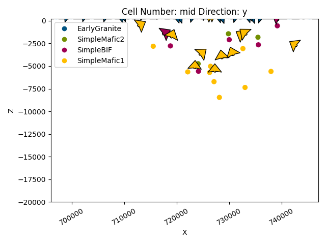
<gempy_viewer.modules.plot_2d.visualization_2d.Plot2D object at 0x7f919f1713c0>

Creating grid

First we need to define the location of the devices. For this example we can make a map:

grav_res = 20
X = np.linspace(7.050000e+05, 747000, grav_res)
Y = np.linspace(6863000, 6925000, grav_res)
Z = 300
xyz = np.meshgrid(X, Y, Z)
xy_ravel = np.vstack(list(map(np.ravel, xyz))).T
xy_ravel

array([[7.05000000e+05, 6.86300000e+06, 3.00000000e+02],
       [7.07210526e+05, 6.86300000e+06, 3.00000000e+02],
       [7.09421053e+05, 6.86300000e+06, 3.00000000e+02],
       ...,
       [7.42578947e+05, 6.92500000e+06, 3.00000000e+02],
       [7.44789474e+05, 6.92500000e+06, 3.00000000e+02],
       [7.47000000e+05, 6.92500000e+06, 3.00000000e+02]])

We can see the location of the devices relative to the model data:

gpv.plot_2d(geo_model, direction='z', show=False)
plt.scatter(xy_ravel[:, 0], xy_ravel[:, 1], s=1)
plt.show()

Now we need to create the grid centered on the devices (see: https://github.com/cgre-aachen/gempy/blob/master/notebooks/tutorials/ch1-3-Grids.ipynb)

geo_model.set_centered_grid(xy_ravel, resolution=[10, 10, 15], radius=5000)

gp.set_centered_grid(
    grid=geo_model.grid,
    centers=xy_ravel,
    resolution=np.array([10, 10, 15]),
    radius=np.array([5000, 5000, 5000])
)

Active grids: ['centered']

CenteredGrid(centers=array([[7.05000000e+05, 6.86300000e+06, 3.00000000e+02],
       [7.07210526e+05, 6.86300000e+06, 3.00000000e+02],
       [7.09421053e+05, 6.86300000e+06, 3.00000000e+02],
       ...,
       [7.42578947e+05, 6.92500000e+06, 3.00000000e+02],
       [7.44789474e+05, 6.92500000e+06, 3.00000000e+02],
       [7.47000000e+05, 6.92500000e+06, 3.00000000e+02]]), resolution=array([10, 10, 15]), radius=array([5000, 5000, 5000]), kernel_grid_centers=array([[-5000.        , -5000.        ,  -300.        ],
       [-5000.        , -5000.        ,  -360.        ],
       [-5000.        , -5000.        ,  -383.36972966],
       ...,
       [ 5000.        ,  5000.        , -3407.68480754],
       [ 5000.        ,  5000.        , -4618.11403801],
       [ 5000.        ,  5000.        , -6300.        ]]), left_voxel_edges=array([[1709.43058496, 1709.43058496,  -30.        ],
       [1709.43058496, 1709.43058496,  -30.        ],
       [1709.43058496, 1709.43058496,  -11.68486483],
       ...,
       [1709.43058496, 1709.43058496, -435.56428767],
       [1709.43058496, 1709.43058496, -605.21461523],
       [1709.43058496, 1709.43058496, -840.942981  ]]), right_voxel_edges=array([[1709.43058496, 1709.43058496,  -30.        ],
       [1709.43058496, 1709.43058496,  -11.68486483],
       [1709.43058496, 1709.43058496,  -16.23606704],
       ...,
       [1709.43058496, 1709.43058496, -605.21461523],
       [1709.43058496, 1709.43058496, -840.942981  ],
       [1709.43058496, 1709.43058496, -840.942981  ]]))

geo_model.grid.centered_grid.kernel_grid_centers

array([[-5000.        , -5000.        ,  -300.        ],
       [-5000.        , -5000.        ,  -360.        ],
       [-5000.        , -5000.        ,  -383.36972966],
       ...,
       [ 5000.        ,  5000.        , -3407.68480754],
       [ 5000.        ,  5000.        , -4618.11403801],
       [ 5000.        ,  5000.        , -6300.        ]])

Now we need to compute the component tz (see https://github.com/cgre-achen/gempy/blob/master/notebooks/tutorials/ch2-2-Cell_selection.ipynb)

gravity_gradient = gp.calculate_gravity_gradient(geo_model.grid.centered_grid)
gravity_gradient

array([-0.00435884, -0.0035374 , -0.00260207, ..., -0.60455378,
       -0.888396  , -0.98280245])

geo_model.geophysics_input = gp.data.GeophysicsInput(
    tz=gravity_gradient,
    densities=np.array([2.61, 2.92, 3.1, 2.92, 2.61]),
)

Once we have created a gravity interpolator we can call it from compute model as follows:

geo_model.interpolation_options.mesh_extraction = False
sol = gp.compute_model(
    gempy_model=geo_model,
    engine_config=gp.data.GemPyEngineConfig(
        backend=gp.data.AvailableBackends.numpy,
        dtype='float32'
    )
)

grav = sol.gravity

Setting Backend To: AvailableBackends.numpy
Chunking done: 16 chunks
Chunking done: 16 chunks
Chunking done: 16 chunks

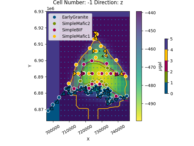
gpv.plot_2d(geo_model, cell_number=[-1], direction=['z'], show_data=False)

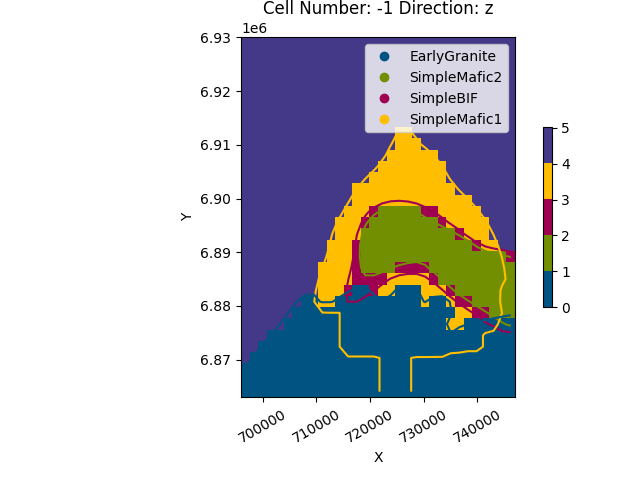
<gempy_viewer.modules.plot_2d.visualization_2d.Plot2D object at 0x7f9191ce7250>

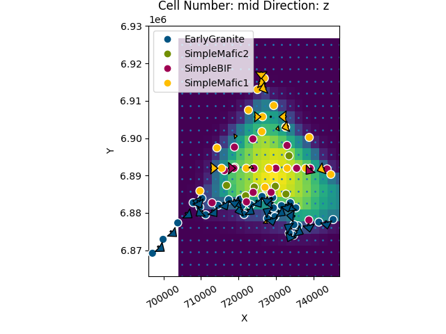
gpv.plot_2d(geo_model, cell_number=['mid'], direction='x')

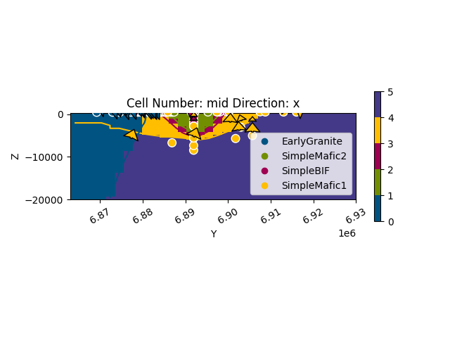
<gempy_viewer.modules.plot_2d.visualization_2d.Plot2D object at 0x7f918fbc49d0>

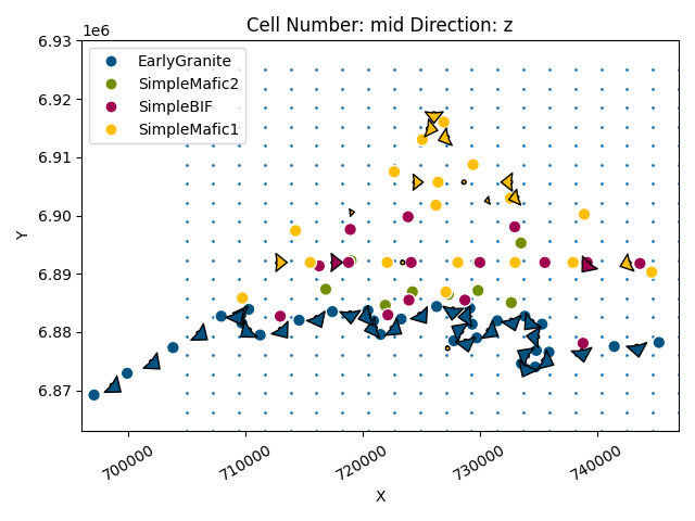
gpv.plot_2d(geo_model, direction=['z'], height=7, show_results=False, show_data=True, show=False)
plt.scatter(xy_ravel[:, 0], xy_ravel[:, 1], s=1)
plt.imshow(sol.gravity.reshape(grav_res, grav_res),
           extent=(xy_ravel[:, 0].min() + (xy_ravel[0, 0] - xy_ravel[1, 0]) / 2,
                   xy_ravel[:, 0].max() - (xy_ravel[0, 0] - xy_ravel[1, 0]) / 2,
                   xy_ravel[:, 1].min() + (xy_ravel[0, 1] - xy_ravel[30, 1]) / 2,
                   xy_ravel[:, 1].max() - (xy_ravel[0, 1] - xy_ravel[30, 1]) / 2),
           cmap='viridis_r', origin='lower')
plt.show()

Plotting lithologies

If we want to compute the lithologies we will need to create a normal interpolator object as seen in the Chapter 1 of the tutorials

Now we can plot all together (change the alpha parameter to see the gravity overlying):

gpv.plot_2d(geo_model, cell_number=[-1], direction=['z'], show=False,
            kwargs_regular_grid={'alpha': .5})

plt.scatter(xy_ravel[:, 0], xy_ravel[:, 1], s=1)
plt.imshow(grav.reshape(grav_res, grav_res),
           extent=(xy_ravel[:, 0].min() + (xy_ravel[0, 0] - xy_ravel[1, 0]) / 2,
                   xy_ravel[:, 0].max() - (xy_ravel[0, 0] - xy_ravel[1, 0]) / 2,
                   xy_ravel[:, 1].min() + (xy_ravel[0, 1] - xy_ravel[30, 1]) / 2,
                   xy_ravel[:, 1].max() - (xy_ravel[0, 1] - xy_ravel[30, 1]) / 2),
           cmap='viridis_r', origin='lower', alpha=.8)
cbar = plt.colorbar()
cbar.set_label(r'$\mu$gal')
plt.show()

# sphinx_gallery_thumbnail_number = -2