Note
Go to the end to download the full example code.
Getting Started
Welcome to our introductory notebook on GemPy! Here, we will cover the essentials of GemPy, introducing you to the core concepts of geomodeling and demonstrating how you can leverage these to create your own geological models. We will guide you through building a model from scratch, based on a conceptual 2D cross-section with boreholes. This simple example will highlight key workflow steps and structural features that GemPy can model.
Installation
Setting Up Our Environment: Importing Libraries
To work with Python packages in our notebook, we need to import them first. Let’s start with that. In the following cell, we will import GemPy and its GemPy viewer module, which we will be using extensively. Additionally, we will use NumPy for various functions, as well as Matplotlib and some of its specific modules/functions for visualizing our data and results in 2D and 3D.
Set environmental variable DEFAULT_BACKEND = PYTORCH
import os

os.environ["DEFAULT_BACKEND"] = "PYTORCH"

# Importing GemPy and viewer
import gempy as gp
import gempy_viewer as gpv

# Auxiliary libraries
import numpy as np
import matplotlib.pyplot as plt
import matplotlib.image as mpimg

# sphinx_gallery_thumbnail_number = 11
Main Classes and Objects in GemPy
GemPy uses Python classes and objects to store and manipulate the data used for modeling. This object-oriented approach helps make the code more modular, reusable, and easier to understand. Each class represents a different aspect of the geological modeling process, and objects are instances of these classes that contain specific data and methods to operate on that data.
Here are the main data classes:
Setting Up a Model: Initializing Objects and Input Data
Before computing a geological model, we need to set up the relevant objects and input data on which the model will be based. Data can be input in various ways. One way is to start from scratch and manually input surface points and orientations. Another way is to import existing data from a file, such as a CSV. Here, we will start with the first method to showcase the essential elements and rules needed to build a model in GemPy.
Starting a Model from Scratch Based on a Cross-Section
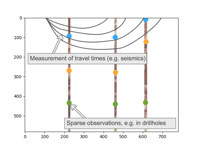
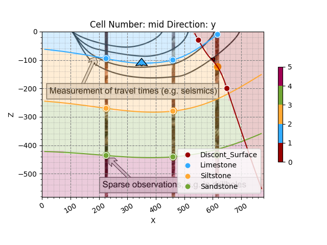
This first example will be based on a conceptual cross-section that includes data from three boreholes in a line. Let’s start by loading the image of this cross-section and plotting it using Matplotlib. For this example, we assume that the size of the image corresponds to the real extent of the data. We will see that extent in the plot and also return it by looking at the shape of the image file:
(582, 780)
OK, so we will base our model creation on this cross-section. Let’s get started. To initialize our model, we create a gempy.Model object. This object will contain all other data structures and necessary functionality. Here’s what we will do:
Name the Model: Assign a name to our model.
Define Extent: Specify the extent in x, y, and z. The extent should make sense depending on your use case and should enclose all relevant data in a representative space. For this example, we align the extent with the cross-section we imported:
X is parallel to the section.
Y is perpendicular. Since we have no data along y, a narrow extent makes sense. We choose an extent of 400, defining it as -200 to 200, placing the cross-section at y=0 (in the middle).
Z representing depth, takes a negative value since we are modeling the subsurface.
Initialize Structural Framework: Set up a default structural framework.
- Define either resolution or refinement: In GemPy 3, you can use either regular grids or octrees.
Regular grids: Define a resolution (and refinement=None). A medium resolution of 50x50x50, for example, results in 125,000 voxels. Model voxels are prisms, not cubes, so resolution can differ from extent. Avoid exceeding 100 cells in each direction (1,000,000 voxels) to prevent high computational costs.
Octrees: Define a level of refinement (and resolution=None). Higher refinement levels increase computational costs.
Note on choice of modeling grids
Which type of grid is used depends on the use case. Note that as of the current version of GemPy 3, the rendering of surfaces uses dual-contouring, which is based on octrees. So even if you choose regular grids, octree-based computing will be executed additionally in order to render the surfaces in 3D.
geo_model = gp.create_geomodel(
    project_name='Model1',
    extent=[0, 780, -200, 200, -582, 0],
    resolution=(50, 50, 50),
    # refinement=4, # We will use octrees
    structural_frame=gp.data.StructuralFrame.initialize_default_structure()
)
The geo_model Object
The gempy.core.data.GeoModel object we just initialized contains all the essential information for constructing our model,
such as the parameters defined above,
and the input data we will introduce further below. You can access different types of information by accessing the attributes. For instance, you
can retrieve the coordinates of our modeling grid as follows:
Grid(values=array([[   7.8 , -196.  , -576.18],
       [   7.8 , -196.  , -564.54],
       [   7.8 , -196.  , -552.9 ],
       ...,
       [ 772.2 ,  196.  ,  -29.1 ],
       [ 772.2 ,  196.  ,  -17.46],
       [ 772.2 ,  196.  ,   -5.82]], shape=(125000, 3)), length=array([], dtype=float64), _octree_grid=None, _dense_grid=RegularGrid(resolution=array([50, 50, 50]), extent=array([   0.,  780., -200.,  200., -582.,    0.]), values=array([[   7.8 , -196.  , -576.18],
       [   7.8 , -196.  , -564.54],
       [   7.8 , -196.  , -552.9 ],
       ...,
       [ 772.2 ,  196.  ,  -29.1 ],
       [ 772.2 ,  196.  ,  -17.46],
       [ 772.2 ,  196.  ,   -5.82]], shape=(125000, 3)), mask_topo=array([], shape=(0, 3), dtype=bool), _transform=None, _base_resolution=array([2, 2, 2])), _custom_grid=None, _topography=None, _sections=None, _centered_grid=None, _transform=None, _octree_levels=-1)
The geo_model object also contains the structural frame of our model, i.e., information about our main structural groups (also referred to as series or stacks in our model), and their sequential and geological relationships with one another. Each group can contain several elements, which can be surfaces representing the bottom interfaces of lithological units or fault planes. Each structural group also has a relation type that defines the relation of the structural elements to others. The relation type is ‘erode’ by default but can also be ‘onlap’ or ‘fault’ (more about this later). The structural frame also contains information about fault relationships, i.e., which elements are affected by which faults. Let’s look at our default structural frame:
As you can see, by default, there is one element called ‘surface 1’ and no faults. However, by default, GemPy actually not only starts off with this ‘surface 1’ but also a ‘basement’ unit which is always present. We can see this using the following function:
[Element(
    name=surface1,
    color=#015482,
    is_active=True
), Element(
    name=basement,
    color=#9f0052,
    is_active=True
)]
We can also rename our structural elements and assign colors as needed. This will later become relevant for the legend in our plots of the data and generated model. Let’s assume we already know our uppermost surface, ‘surface 1,’ is a limestone unit. Let’s also ensure it is represented by the same color as displayed in the cross-section. For this, we input hex color codes.
geo_model.structural_frame.structural_elements[0].color = '#33ABFF'  # Set 'surface 1' color to blue.
geo_model.structural_frame.structural_elements[1].color = '#570987'  # Set basement color to purple.

geo_model.structural_frame.structural_elements[0].name = 'Limestone'  # Renaming 'surface 1' to 'Limestone'.
geo_model.structural_frame.structural_elements[0]
geo_model.structural_frame.structural_groups[0].name = 'Deposit. Series'
Manually Inputting Data
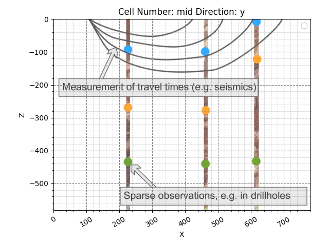
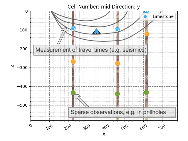
Now that the geo_model object has been created and our first structural element renamed, we can start inputting data by reading it from the cross-section. We start with location points that represent the boundaries between two lithological units. Let’s look at the cross-section again. This time we use a gempy_viewer function to create a plot that can include the cross-section image, as well as data in the object geo_model - which is for now empty but we will start adding data next. Let’s also add a grid to better read the location of points.
The image cross-section indicates that there are three lithological boundaries, with one dot for each boundary shown in the first two boreholes. The third borehole doesn’t go as deep and only provides one dot, i.e., information about the first boundary. These dots represent the location of a boundary surface in depth. Remember also that in GemPy, each surface represents the bottom of the unit it is assigned to.
p2d = gpv.plot_2d(geo_model, show=False)
p2d.axes[0].imshow(img, origin='upper', alpha=.8, extent=(0, 780, -582, 0))

# Enable grid with minor ticks
p2d.axes[0].grid(which='both')  # Enable both major and minor grids
p2d.axes[0].minorticks_on()  # Enable minor ticks

# Customize the appearance of the grid if needed
p2d.axes[0].grid(which='major', linestyle='--', linewidth='0.8', color='gray')
p2d.axes[0].grid(which='minor', linestyle=':', linewidth='0.4', color='gray')

plt.show()
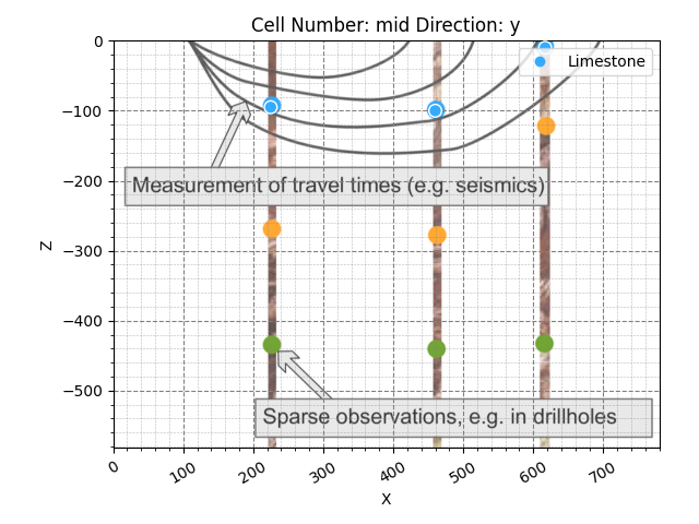
Looking at the plot, we can read the location of the surface points and start adding them to our geo_model object. For now, let’s focus on only the uppermost layer, the limestone, with its bottom boundary represented by the blue dots. Using the function add_surface_points, we can start adding the positional points to our geo_model object. Let’s start with only one. From looking at the plot, the first blue point seems to be located at approximately 250 in the x direction and around 95 meters in depth. Since we assume the section to be at y=0, we can leave y as 0. We can input that as follows: %%
gp.add_surface_points(
    geo_model=geo_model,
    x=[225],
    y=[0],
    z=[-95],
    elements_names=['Limestone']
)
Now let’s plot the data with the section and see how we did:
p2d = gpv.plot_2d(geo_model, show=False)
p2d.axes[0].imshow(img, origin='upper', alpha=.8, extent=(0, 780, -582, 0))

# Enable grid with minor ticks
p2d.axes[0].grid(which='both')  # Enable both major and minor grids
p2d.axes[0].minorticks_on()  # Enable minor ticks

# Customize the appearance of the grid if needed
p2d.axes[0].grid(which='major', linestyle='--', linewidth='0.8', color='gray')
p2d.axes[0].grid(which='minor', linestyle=':', linewidth='0.4', color='gray')

plt.show()

Great! As you can see, the data point we entered sits right on top of the blue dot on the borehole. Now let’s do the same for the other borehole dots. Conveniently, we can use the same function to add several points at a time:
gp.add_surface_points(
    geo_model=geo_model,
    x=[460, 617],
    y=[0, 0],
    z=[-100, -10],
    elements_names=['Limestone', 'Limestone']
)

p2d = gpv.plot_2d(geo_model, show=False)
p2d.axes[0].imshow(img, origin='upper', alpha=.8, extent=(0, 780, -582, 0))

# Enable grid with minor ticks
p2d.axes[0].grid(which='both')  # Enable both major and minor grids
p2d.axes[0].minorticks_on()  # Enable minor ticks

# Customize the appearance of the grid if needed
p2d.axes[0].grid(which='major', linestyle='--', linewidth='0.8', color='gray')
p2d.axes[0].grid(which='minor', linestyle=':', linewidth='0.4', color='gray')

plt.show()
Minimum Data for Model Computation
Ok, good! Now we have added the position of the bottom of this top layer for each borehole. But is this enough to compute our first layer? Well, no. GemPy’s approach is based on an implicit interpolation method that requires the following minimum data:
Two surface points for at least one surface in a structural group/series
One orientation per structural group/series
Thanks to GemPy’s global interpolation approach, once you have one surface defined by two surface points and an orientation in a structural group, you can add more surfaces (in the same group) with the minimum of one surface point, as it will now take its orientation information from the other surface.
So, we are missing an orientation. Let’s go ahead and add one. It seems that we can assume a horizontal orientation between the first two surface points (apparent, as we have no information about the y-direction). Let’s add a corresponding orientation using the function add_orientations:
gp.add_orientations(
    geo_model=geo_model,
    x=[350],
    y=[0],
    z=[-120],
    elements_names=['Limestone'],
    pole_vector=[np.array([0, 0, 1])]
)

p2d = gpv.plot_2d(geo_model, show=False)
p2d.axes[0].imshow(img, origin='upper', alpha=.8, extent=(0, 780, -582, 0))

# Enable grid with minor ticks
p2d.axes[0].grid(which='both')  # Enable both major and minor grids
p2d.axes[0].minorticks_on()  # Enable minor ticks

# Customize the appearance of the grid if needed
p2d.axes[0].grid(which='major', linestyle='--', linewidth='0.8', color='gray')
p2d.axes[0].grid(which='minor', linestyle=':', linewidth='0.4', color='gray')

plt.show()
Alright, now we actually have sufficient input data to compute the first version of our model. Let’s go ahead and do that using compute_model:
geo_model.update_transform(gp.data.GlobalAnisotropy.NONE)
gp.compute_model(geo_model, engine_config=gp.data.GemPyEngineConfig())
Setting Backend To: AvailableBackends.PYTORCH
GPU requested but unavailable; falling back to CPU (GEMPY_GPU_FALLBACK=True)
Setting Backend To: AvailableBackends.PYTORCH
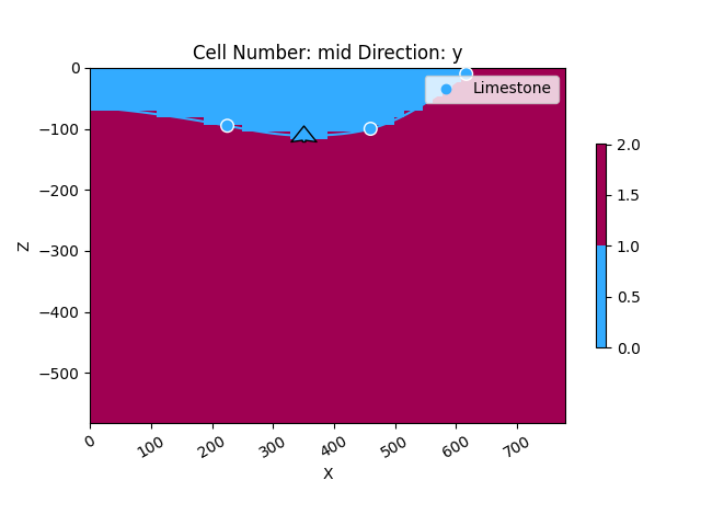
Now, the model has been computed and is ready to be visualized. Let’s see what it looks like in a 2D section:
2D visualization:
gpv.plot_2d(geo_model, cell_number='mid')
<gempy_viewer.modules.plot_2d.visualization_2d.Plot2D object at 0x7f5820e19350>
We can also plot it together with our cross-section image. By using transparency on the cross-section image, we can overlay it over the 2D model visualization.
p2d = gpv.plot_2d(geo_model, show=False)
p2d.axes[0].imshow(img, origin='upper', alpha=.8, extent=(0, 780, -582, 0))

# Enable grid with minor ticks
p2d.axes[0].grid(which='both')  # Enable both major and minor grids
p2d.axes[0].minorticks_on()  # Enable minor ticks

# Customize the appearance of the grid if needed
p2d.axes[0].grid(which='major', linestyle='--', linewidth='0.8', color='gray')
p2d.axes[0].grid(which='minor', linestyle=':', linewidth='0.4', color='gray')

plt.show()
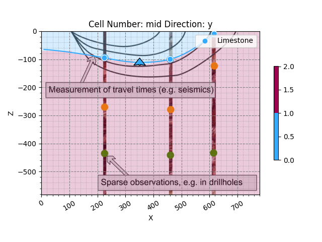
You can see how the computed interface runs through the points we defined and is furthermore determined by the one orientation we placed. Now, let’s look at our 3D model:
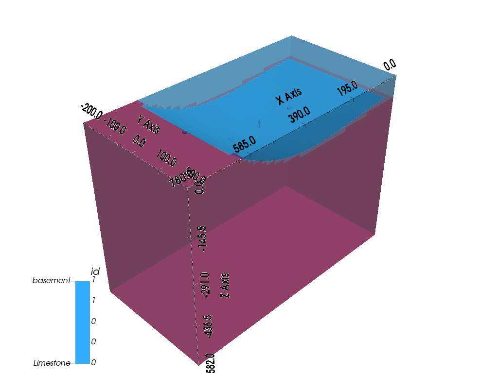
3D visualization:
gpv.plot_3d(geo_model, show_surfaces=True, image=False)
<gempy_viewer.modules.plot_3d.vista.GemPyToVista object at 0x7f5820c4e7b0>
Very good, we have successfully computed the first iteration of our model including one lithological interface. You could now go ahead and fine-tune the model by adding further points or orientations. For now, let’s continue.
About Scalar Fields
GemPy’s global interpolation approach uses scalar fields to compute models. Each structural group or series has its own scalar field, which is defined by the data input to all of its elements and at least the minimum data mentioned above. Given that alone, a scalar field will already be created “globally”, i.e., for the full extent of the modeling space. The defined surface follows one value along that field as an isosurface. A separate structural element will follow a different isosurface, and once you input additional points and orientations, the scalar field will be altered accordingly.
As mentioned, each structural group has its own scalar field. These can be combined to achieve more complex structures and relationships, as we will see later.
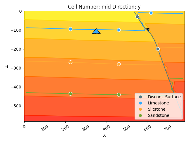
Let’s take a look at the current scalar field for our current group by plotting it in 2D. Keep it in mind as we go ahead and add additional elements and data.
p2d = gpv.plot_2d(
    model=geo_model,
    series_n=0,
    show_data=True,
    show_scalar=True,
    show_lith=False
)

plt.show()

Adding a Second Lithological Unit
To add another unit to our model, we can define it as another structural element and then append it to our geo_model object. We do this for the second unit in the following steps. See how we can already give it a name (let’s assume this is a siltstone now), a color corresponding to the dot colors in the cross-section, as well as define surface points and orientations. By appending it to structural_groups[0], we are adding it to our first (and currently only) structural group/series, i.e., it will be in the same stack as our limestone.
element2 = gp.data.StructuralElement(
    name='Siltstone',
    color='#FFA833',  # color=next(geo_model.structural_frame.color_generator),
    surface_points=gp.data.SurfacePointsTable.from_arrays(
        x=np.array([460]),
        y=np.array([0]),
        z=np.array([-280]),
        names='Siltstone'
    ),
    orientations=gp.data.OrientationsTable.initialize_empty()
)

geo_model.structural_frame.structural_groups[0].append_element(element2)
Now, we can see that this siltstone unit is part of our structural frame. Note below, that it has by default been added below the limestone. The order of structural elements within one group only affects the default color assigned. We recommend being consistent in the way you choose to order them, and to order them in accordance with geological age. The order of structural groups actually represents geological time relationships, with groups at the top being the youngest and lower ones being older. This, together with their StackRelationType, decides how they affect each other via their individual scalar fields, as we will see later.
gp.compute_model(geo_model, engine_config=gp.data.GemPyEngineConfig())
Setting Backend To: AvailableBackends.PYTORCH
GPU requested but unavailable; falling back to CPU (GEMPY_GPU_FALLBACK=True)
Setting Backend To: AvailableBackends.PYTORCH
p2d = gpv.plot_2d(geo_model, cell='mid', show=False)
p2d.axes[0].imshow(img, origin='upper', alpha=.8, extent=(0, 780, -582, 0))

# Enable grid with minor ticks
p2d.axes[0].grid(which='both')  # Enable both major and minor grids
p2d.axes[0].minorticks_on()  # Enable minor ticks

# Customize the appearance of the grid if needed
p2d.axes[0].grid(which='major', linestyle='--', linewidth='0.8', color='gray')
p2d.axes[0].grid(which='minor', linestyle=':', linewidth='0.4', color='gray')

plt.show()
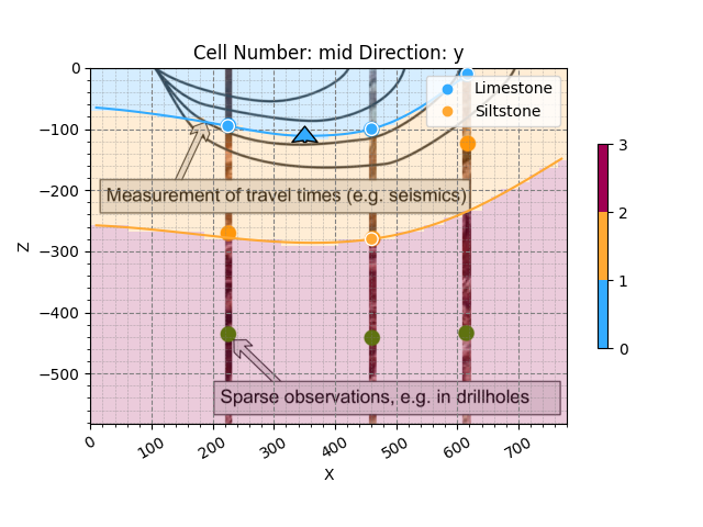
The 2D visualization of our updated model now shows that the next surface follows the respective point we added. Based on the implicit modeling approach GemPy uses, given this sparse information we have put in, the siltstone bottom interface otherwise follows the course and orientation of the limestone we defined earlier. This is due to the scalar field which was defined by the data input for the structural group as a whole. In our 2D plot, we can see that this fits quite well with the first borehole, too. Still, let’s add the remaining point, and while we are at it, let’s also add the third lithological unit marked in green.
First, we add the two missing points to the Siltstone
gp.add_surface_points(
geo_model=geo_model,
x=[225],
y=[0],
z=[-270],
elements_names=['Siltstone']
)
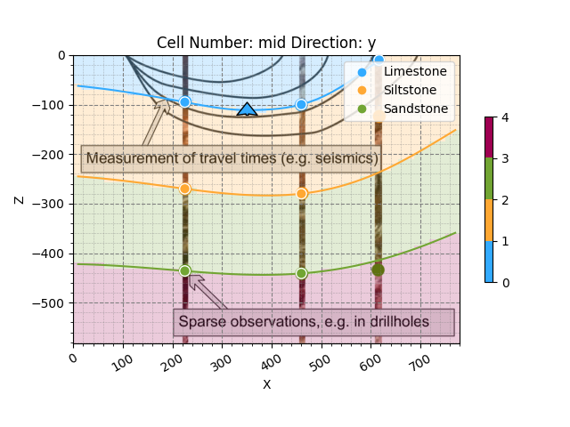
element3 = gp.data.StructuralElement(
name='Sandstone',
color='#72A533', # next(geo_model.structural_frame.color_generator),
surface_points=gp.data.SurfacePointsTable.from_arrays(
x=np.array([225, 460]),
y=np.array([0, 0]),
z=np.array([-436, -441]),
names='Sandstone'
),
orientations=gp.data.OrientationsTable.initialize_empty()
)
geo_model.structural_frame.structural_groups[0].append_element(element3)
Setting Backend To: AvailableBackends.PYTORCH
GPU requested but unavailable; falling back to CPU (GEMPY_GPU_FALLBACK=True)
Setting Backend To: AvailableBackends.PYTORCH
p2d = gpv.plot_2d(geo_model, show=False)
p2d.axes[0].imshow(img, origin='upper', alpha=.8, extent=(0, 780, -582, 0))

# Enable grid with minor ticks
p2d.axes[0].grid(which='both')  # Enable both major and minor grids
p2d.axes[0].minorticks_on()  # Enable minor ticks

# Customize the appearance of the grid if needed
p2d.axes[0].grid(which='major', linestyle='--', linewidth='0.8', color='gray')
p2d.axes[0].grid(which='minor', linestyle=':', linewidth='0.4', color='gray')

plt.show()
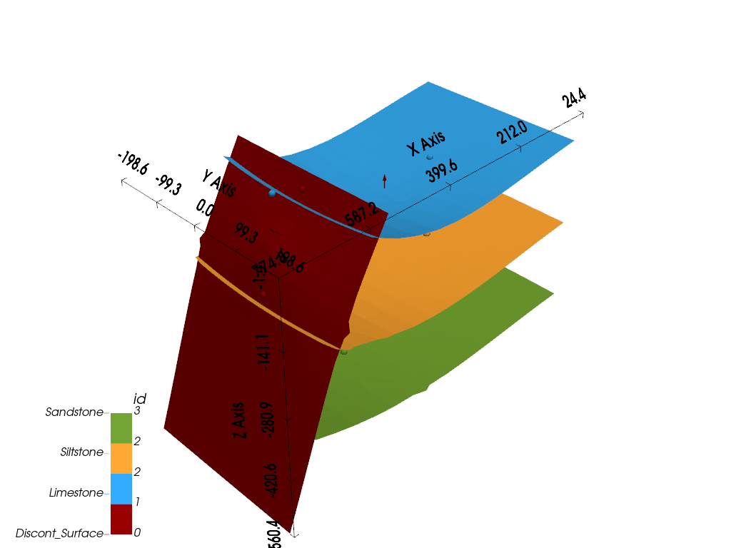
3D visualization:
gpv.plot_3d(geo_model, show_surfaces=True, image=False)
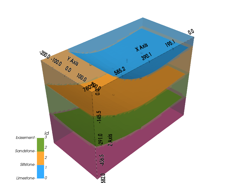
<gempy_viewer.modules.plot_3d.vista.GemPyToVista object at 0x7f5820e0ca50>
Discontinuities: Combining Scalar Fields
Now that we have created all the lithological units and added all the surface points we got from the boreholes, we have created a very simple geological model. However, geological scenarios are usually more complex. In GemPy, you can not only combine numerous surface points and orientations to create elaborate structures but also create various structural groups that affect each other through combinations of their scalar fields. In the following part, we will look at the right side of our cross-section, where we only have limited data, and see how we can add a new structural group to create various types of discontinuities, and with that, possibly even meaningful alternative model hypotheses.
So, let’s define another structural element that will serve to showcase the different types of discontinuities we can implement in GemPy:
element_discont = gp.data.StructuralElement(
    name='Discont_Surface',
    color='#990000',  # next(geo_model.structural_frame.color_generator),
    surface_points=gp.data.SurfacePointsTable.from_arrays(
        x=np.array([550, 650]),
        y=np.array([0, 0]),
        z=np.array([-30, -200]),
        names='Discont_Surface'
    ),
    orientations=gp.data.OrientationsTable.from_arrays(
        x=np.array([600]),
        y=np.array([0]),
        z=np.array([-100]),
        G_x=np.array([.3]),
        G_y=np.array([0]),
        G_z=np.array([.3]),
        names='Discont_Surface'
    )
)
To place the discontinuity element in a separate structural group, we need to create one. This is what we do next. Note that we directly add the element to the group as we create it, and we define the group’s structural relation type as the default ‘erode’. We can then insert the group into the structural frame.
group_discont = gp.data.StructuralGroup(
    name='Discontinuity',
    elements=[element_discont],
    structural_relation=gp.data.StackRelationType.ERODE,
)

# Insert the fault group into the structural frame:
geo_model.structural_frame.insert_group(0, group_discont)
Let’s take a quick look at the state of our structural frame.
We can now see the two different structural groups: the default one containing the deposition series, and the group containing the discontinuity. Let’s go ahead and compute the model. Once the model has been computed, we can plot the scalar fields of both structural groups independently.
gp.compute_model(geo_model, engine_config=gp.data.GemPyEngineConfig())
Setting Backend To: AvailableBackends.PYTORCH
GPU requested but unavailable; falling back to CPU (GEMPY_GPU_FALLBACK=True)
Setting Backend To: AvailableBackends.PYTORCH
p2d = gpv.plot_2d(
    model=geo_model,
    series_n=1,  # This setting will now plot the scalar field used for the fault
    show_data=True,
    show_scalar=True,
    show_lith=False
)

plt.show()
p2d = gpv.plot_2d(
    model=geo_model,
    series_n=0,  # This setting will plot the scalar field used for the discontinuity.
    show_data=True,
    show_scalar=True,
    show_lith=False
)

plt.show()
We now have two very different scalar fields. Note how they are each defined by the input data assigned to their respective structural elements. Multiple scalar fields in GemPy influence each other depending on (1) their order and (2) their StackRelationType. The latter defines how a younger (upper) structural group will relate to the older (lower) structural groups and possibly affect their scalar field.
The parameter StackRelationType can take the following values:
BASEMENT: Treats all lower groups as the basement.
ERODE: Defines erosive contact/unconformity.
ONLAP: Defines the younger group to be onlapping onto the older groups.
FAULT: Defines the group to be a fault.
We will now take a look at each of these relation types except for the basement type.
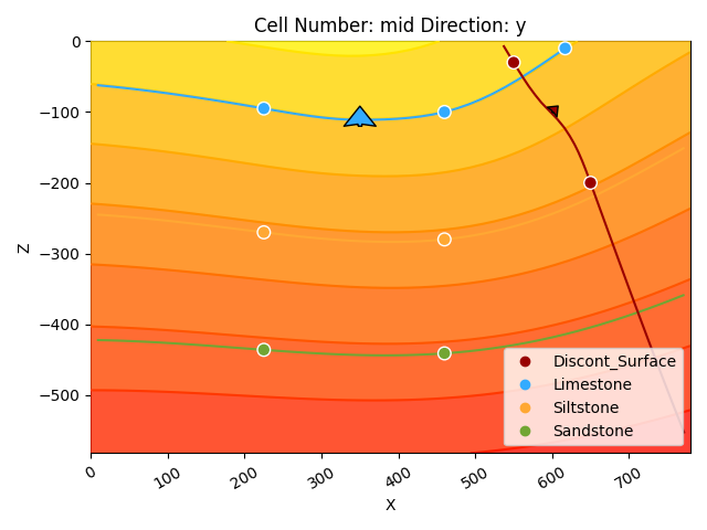
Erosive Contact
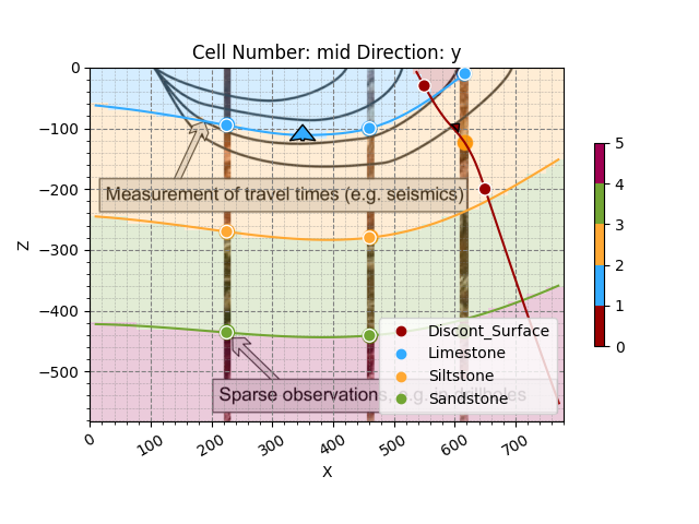
For this, we don’t have to change anything now, as we already set the StackRelationType to be ERODE. If we now plot it, we will see how this younger structural group erodes all older elements and basically “cuts them out” in our model.
p2d = gpv.plot_2d(geo_model, show=False)
p2d.axes[0].imshow(img, origin='upper', alpha=.8, extent=(0, 780, -582, 0))

# Enable grid with minor ticks
p2d.axes[0].grid(which='both')  # Enable both major and minor grids
p2d.axes[0].minorticks_on()  # Enable minor ticks

# Customize the appearance of the grid if needed
p2d.axes[0].grid(which='major', linestyle='--', linewidth='0.8', color='gray')
p2d.axes[0].grid(which='minor', linestyle=':', linewidth='0.4', color='gray')

plt.show()
3D visualization:
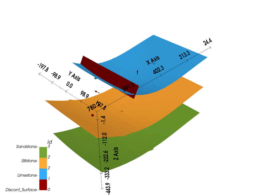
gpv.plot_3d(geo_model, show_surfaces=True, image=False, show_lith=False)
<gempy_viewer.modules.plot_3d.vista.GemPyToVista object at 0x7f5820e9ae90>
We can see how all units of the depositional series stop at the contact with the new discontinuity group. However, this doesn’t look quite right, and it in particular doesn’t fit the surface point that was observed in the third borehole. So let’s try another relation type.
Onlapping
Let’s change the relation type from ERODE to ONLAP to achieve a different type of discontinuity and then plot it.
geo_model.structural_frame.structural_groups[0].structural_relation = gp.data.StackRelationType.ONLAP
gp.compute_model(geo_model, engine_config=gp.data.GemPyEngineConfig())
Setting Backend To: AvailableBackends.PYTORCH
GPU requested but unavailable; falling back to CPU (GEMPY_GPU_FALLBACK=True)
Setting Backend To: AvailableBackends.PYTORCH
p2d = gpv.plot_2d(geo_model, show=False)
p2d.axes[0].imshow(img, origin='upper', alpha=.8, extent=(0, 780, -582, 0))

# Enable grid with minor ticks
p2d.axes[0].grid(which='both')  # Enable both major and minor grids
p2d.axes[0].minorticks_on()  # Enable minor ticks

# Customize the appearance of the grid if needed
p2d.axes[0].grid(which='major', linestyle='--', linewidth='0.8', color='gray')
p2d.axes[0].grid(which='minor', linestyle=':', linewidth='0.4', color='gray')

plt.show()
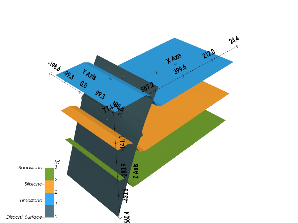
3D visualization:
gpv.plot_3d(geo_model, show_surfaces=True, image=False, show_lith=False)
<gempy_viewer.modules.plot_3d.vista.GemPyToVista object at 0x7f5820e19ba0>
Now the unit defined as part of the discontinuity group is onlapping onto the uppermost surface of the default group and ends there. This also doesn’t really make sense considering the data given, so let’s try the last relation type.
Faults
Let’s change the relation type to FAULT and plot the results. For a fault, we also need to make use of the function set_is_fault.
geo_model.structural_frame.structural_groups[0].structural_relation = gp.data.StackRelationType.FAULT
gp.set_is_fault(
    frame=geo_model.structural_frame,
    fault_groups=['Discontinuity']
)
See that the fault relations field in the structural frame now indicates that the fault affects the default formation, i.e., offsets it. Let’s compute our model including the fault and see what that looks like.
gp.compute_model(geo_model, engine_config=gp.data.GemPyEngineConfig())
Setting Backend To: AvailableBackends.PYTORCH
GPU requested but unavailable; falling back to CPU (GEMPY_GPU_FALLBACK=True)
Setting Backend To: AvailableBackends.PYTORCH
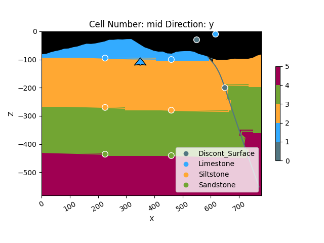
p2d = gpv.plot_2d(geo_model, show=False)
p2d.axes[0].imshow(img, origin='upper', alpha=.8, extent=(0, 780, -582, 0))

# Enable grid with minor ticks
p2d.axes[0].grid(which='both')  # Enable both major and minor grids
p2d.axes[0].minorticks_on()  # Enable minor ticks

# Customize the appearance of the grid if needed
p2d.axes[0].grid(which='major', linestyle='--', linewidth='0.8', color='gray')
p2d.axes[0].grid(which='minor', linestyle=':', linewidth='0.4', color='gray')

plt.show()
3D visualization:
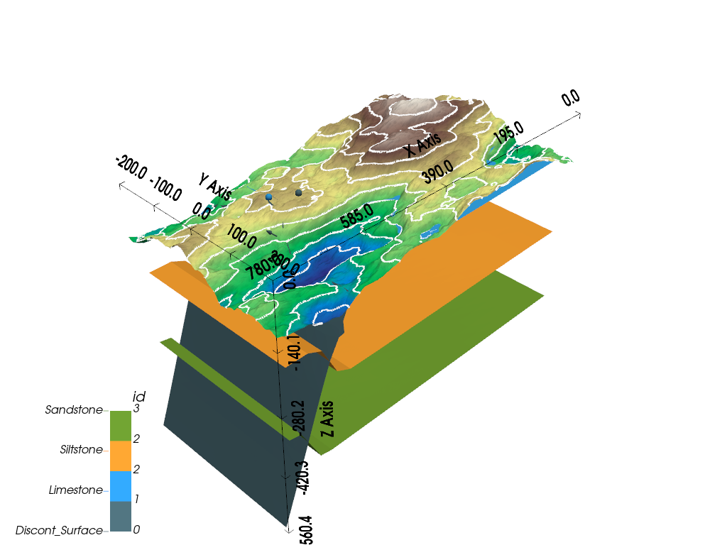
gpv.plot_3d(geo_model, show_surfaces=True, image=False, show_lith=False)
<gempy_viewer.modules.plot_3d.vista.GemPyToVista object at 0x7f58355708a0>
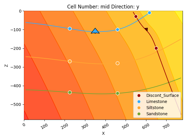
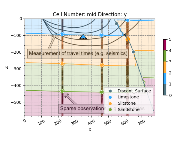
In the 2D and 3D visualizations, we can now see how the insertion of a fault has created a viable alternative hypothesis that fits the original data in the cross-section. Instead of a larger syncline structure and upward-bending of the whole depositional series, we can now explain the shallower depth of the limestone in the third borehole by the effects of a reverse fault. In this model realization, all lithological units are oriented near-horizontal but are offset by the fault. Note that in GemPy, the degree of offset is defined by the location of the surface points on each side. If there is no data on one side of a fault, a very large offset will be assumed.
Note also that by implementing a fault, the scalar field of the depositional series has been affected by the offset.
p2d = gpv.plot_2d(
    model=geo_model,
    series_n=1,  # This will plot the scalar field used for the fault
    show_data=True,
    show_scalar=True,
    show_lith=False
)

plt.show()
Topography and Geological Maps
In GemPy, we can add more grid types for different purposes, such as to add topography to our model. In this following section, we will exemplify this by creating a random topography grid which allows us to intersect the surfaces as well as compute a high-resolution geological map. GemPy has a built-in function to generate random topography. After executing it, a topography grid will be added to the geo_model. It can be directly visualized in 2D and 3D.
GemPy offers built-in tools to manage topographic data through gdal. For demonstration, we’ll create a random topography:
gp.set_topography_from_random(
    grid=geo_model.grid,
    fractal_dimension=1.9,
    d_z=np.array([-150, 0]),
    topography_resolution=np.array([200, 200])
)
Active grids: GridTypes.DENSE|TOPOGRAPHY|NONE

Topography(_regular_grid=RegularGrid(resolution=array([50, 50, 50]), extent=array([   0.,  780., -200.,  200., -582.,    0.]), values=array([[   7.8 , -196.  , -576.18],
       [   7.8 , -196.  , -564.54],
       [   7.8 , -196.  , -552.9 ],
       ...,
       [ 772.2 ,  196.  ,  -29.1 ],
       [ 772.2 ,  196.  ,  -17.46],
       [ 772.2 ,  196.  ,   -5.82]], shape=(125000, 3)), mask_topo=array([], shape=(0, 3), dtype=bool), _transform=None, _base_resolution=array([2, 2, 2])), values_2d=array([[[   0.        , -200.        ,  -63.26327528],
        [   0.        , -197.98994975,  -61.5467894 ],
        [   0.        , -195.9798995 ,  -60.99415947],
        ...,
        [   0.        ,  195.9798995 ,  -68.16039394],
        [   0.        ,  197.98994975,  -67.24453096],
        [   0.        ,  200.        ,  -65.52292916]],

       [[   3.91959799, -200.        ,  -63.33157582],
        [   3.91959799, -197.98994975,  -62.41327538],
        [   3.91959799, -195.9798995 ,  -61.30506439],
        ...,
        [   3.91959799,  195.9798995 ,  -67.60038957],
        [   3.91959799,  197.98994975,  -66.94015532],
        [   3.91959799,  200.        ,  -65.53099605]],

       [[   7.83919598, -200.        ,  -64.66310395],
        [   7.83919598, -197.98994975,  -62.84394334],
        [   7.83919598, -195.9798995 ,  -61.72620964],
        ...,
        [   7.83919598,  195.9798995 ,  -67.17841556],
        [   7.83919598,  197.98994975,  -66.6263553 ],
        [   7.83919598,  200.        ,  -66.51928789]],

       ...,

       [[ 772.16080402, -200.        ,  -62.68113264],
        [ 772.16080402, -197.98994975,  -62.31145391],
        [ 772.16080402, -195.9798995 ,  -62.1387962 ],
        ...,
        [ 772.16080402,  195.9798995 ,  -66.04077214],
        [ 772.16080402,  197.98994975,  -65.12253876],
        [ 772.16080402,  200.        ,  -63.73901459]],

       [[ 776.08040201, -200.        ,  -62.53855543],
        [ 776.08040201, -197.98994975,  -61.22243102],
        [ 776.08040201, -195.9798995 ,  -61.06334838],
        ...,
        [ 776.08040201,  195.9798995 ,  -67.17642884],
        [ 776.08040201,  197.98994975,  -66.0493732 ],
        [ 776.08040201,  200.        ,  -64.60645349]],

       [[ 780.        , -200.        ,  -63.05411425],
        [ 780.        , -197.98994975,  -61.28177864],
        [ 780.        , -195.9798995 ,  -60.20599589],
        ...,
        [ 780.        ,  195.9798995 ,  -67.46156424],
        [ 780.        ,  197.98994975,  -66.87958642],
        [ 780.        ,  200.        ,  -65.23496731]]],
      shape=(200, 200, 3)), source=None, values=array([[   0.        , -200.        ,  -63.26327528],
       [   0.        , -197.98994975,  -61.5467894 ],
       [   0.        , -195.9798995 ,  -60.99415947],
       ...,
       [ 780.        ,  195.9798995 ,  -67.46156424],
       [ 780.        ,  197.98994975,  -66.87958642],
       [ 780.        ,  200.        ,  -65.23496731]], shape=(40000, 3)), resolution=(200, 200), raster_shape=())
gpv.plot_2d(geo_model, show_topography=True)
<gempy_viewer.modules.plot_2d.visualization_2d.Plot2D object at 0x7f580c3ee750>
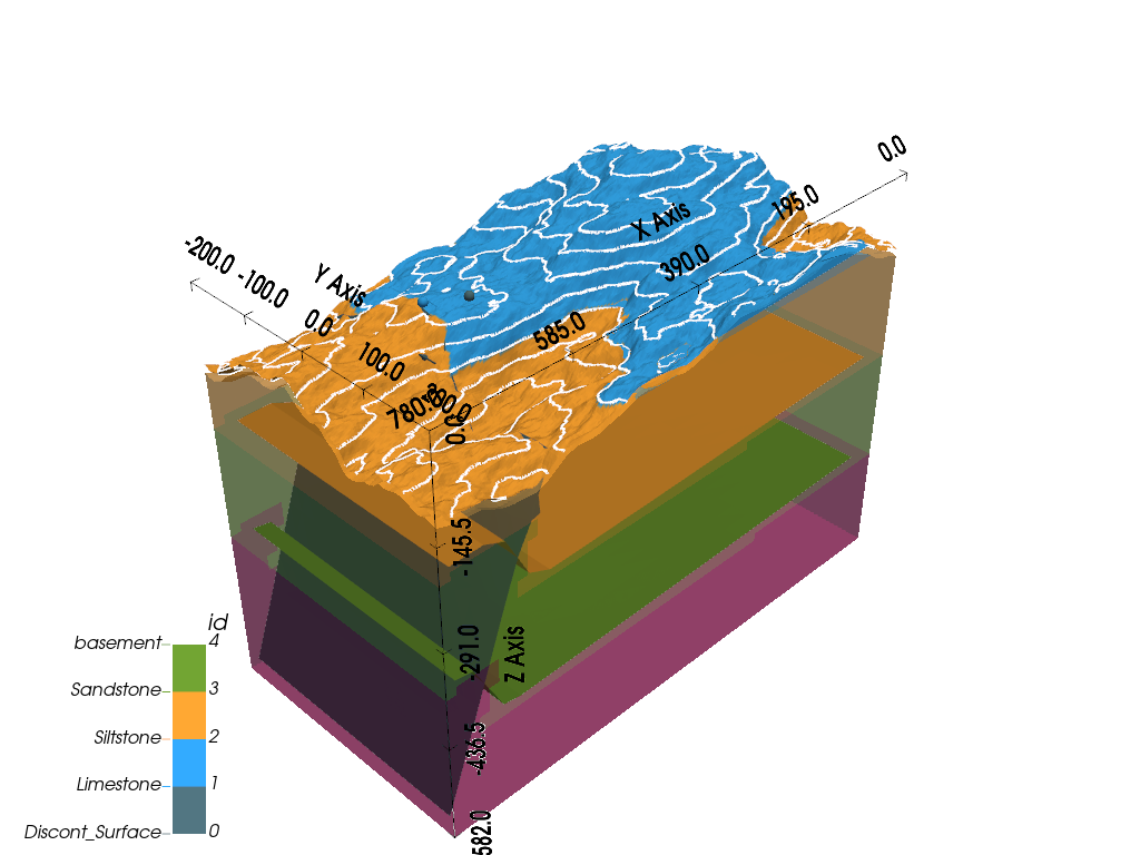
gpv.plot_3d(geo_model, show_surfaces=True, image=False, show_topography=True, show_lith=False)
<gempy_viewer.modules.plot_3d.vista.GemPyToVista object at 0x7f580c34b1d0>
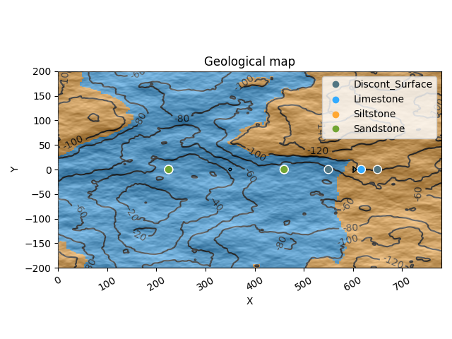
If we now also re-compute our geological model, the generated topography grid will display the lithological units that intersect it, i.e., which outcrop at the surface. We can therefore display a geological map based on our topography and the underlying 3D geological model. To plot a top-down view of this map, you can pass the arguments section_names=[‘topography’] and show_topography=True in the plotting function as shown below.
Setting Backend To: AvailableBackends.PYTORCH
GPU requested but unavailable; falling back to CPU (GEMPY_GPU_FALLBACK=True)
Setting Backend To: AvailableBackends.PYTORCH
gpv.plot_2d(geo_model, section_names=['topography'], show_topography=True)
/opt/buildAgent/work/3a8738c25f60c3c9/venv/lib/python3.14/site-packages/gempy_viewer/API/_plot_2d_sections_api.py:112: UserWarning: Section contacts not implemented yet. We need to pass scalar field for the sections grid
  warnings.warn(

<gempy_viewer.modules.plot_2d.visualization_2d.Plot2D object at 0x7f583564b290>
gpv.plot_3d(geo_model, show_surfaces=True, image=False, show_topography=True)
<gempy_viewer.modules.plot_3d.vista.GemPyToVista object at 0x7f57bfee2be0>
We can now see how the topography displays the color of the lithologies outcropping at the surface, together with topographical contour lines.
While this topography is random, GemPy also has the capability to include real topography files and arrays via the functions set_topography_from_file and set_topography_from_arrays.
Extracting Model Solutions
Once you have built a model, you might not only want to visualize it, but also further analyze it or export it for further utilization. For this, it is good to know that the solutions from modeling are stored in geo_model.solutions and can be returned from there. This includes the following outputs in particular: - geo_model.solutions.dc_meshes: A list of the surface meshes in the model with the location of vertices and edges for each. - geo_model.solutions.raw_arrays: An object containing numerous arrays that define various parts of the model. Of particular importance are the lithology block (lith_block), the fault block (fault_block), and the scalar field matrix (scalar_field_matrix).
Mesh Solutions
Let’s take a quick look at how we can return some key information from geo_model.solutions. Starting with meshes, we can see that the list dc_meshes can be indexed to return specific meshes and their respective vertices or edges. Please note that the order will be the same as in our structural_frame, i.e., the index [0] will return the first and top surface, in our case, the discontinuity surface.
vertices_0 = geo_model.solutions.dc_meshes[0].vertices
edges_0 = geo_model.solutions.dc_meshes[0].edges
print(type(vertices_0), vertices_0, edges_0)
<class 'numpy.ndarray'> [[ 0.45125608 -0.23913328 -0.63074819]
 [ 0.4361575  -0.23913329 -0.58978838]
 [ 0.4511961  -0.20724871 -0.63095396]
 ...
 [ 0.21779507  0.20725281 -0.04149725]
 [ 0.23729301  0.23914443 -0.07938313]
 [ 0.21702129  0.23913719 -0.04242709]] [[  3   1   2]
 [  8   6   3]
 [  9   7   8]
 ...
 [316 314 313]
 [318 323 314]
 [327 325 323]]
We can see that the vertices for this mesh were returned as a Numpy array with values for x, y, and z positions for each vertex. However, the values don’t correspond with our model extent. That is because they have been transformed in GemPy. To return the values corresponding to the original coordinate system, we can invert this transformation as follows:
geo_model.input_transform.apply_inverse(vertices_0)
array([[ 774.78476686, -187.48049221, -559.50657799],
       [ 762.94748262, -187.48050162, -527.3940932 ],
       [ 774.73774175, -162.48298666, -559.66790462],
       ...,
       [ 591.75133532,  162.48620227,  -97.53384549],
       [ 607.03772032,  187.48923477, -127.23637251],
       [ 591.14469153,  187.48355449,  -98.26284214]], shape=(338, 3))
Lithology Block
The lithology block is an array that, for a given model realization/solution, returns the ID of the lithology for each voxel. Note below that the lith_block first returns all values in the shape of one row. You might need to reshape it as shown below. For a regular grid, you can reshape it using the resolution used in geo_model.
lith_block = geo_model.solutions.raw_arrays.lith_block
print(lith_block.shape, lith_block)
(125000,) [5 5 5 ... 3 3 2]
lith_block = lith_block.reshape(50, 50, 50)
print(lith_block.shape, lith_block)
(50, 50, 50) [[[5 5 5 ... 2 2 2]
  [5 5 5 ... 2 2 2]
  [5 5 5 ... 2 2 2]
  ...
  [5 5 5 ... 2 2 2]
  [5 5 5 ... 2 2 2]
  [5 5 5 ... 2 2 2]]

 [[5 5 5 ... 2 2 2]
  [5 5 5 ... 2 2 2]
  [5 5 5 ... 2 2 2]
  ...
  [5 5 5 ... 2 2 2]
  [5 5 5 ... 2 2 2]
  [5 5 5 ... 2 2 2]]

 [[5 5 5 ... 2 2 2]
  [5 5 5 ... 2 2 2]
  [5 5 5 ... 2 2 2]
  ...
  [5 5 5 ... 2 2 2]
  [5 5 5 ... 2 2 2]
  [5 5 5 ... 2 2 2]]

 ...

 [[5 5 5 ... 3 3 2]
  [5 5 5 ... 3 3 2]
  [5 5 5 ... 3 3 2]
  ...
  [5 5 5 ... 3 3 2]
  [5 5 5 ... 3 3 2]
  [5 5 5 ... 3 3 2]]

 [[5 5 5 ... 3 3 2]
  [5 5 5 ... 3 3 2]
  [5 5 5 ... 3 3 2]
  ...
  [5 5 5 ... 3 3 2]
  [5 5 5 ... 3 3 2]
  [5 5 5 ... 3 3 2]]

 [[5 5 5 ... 3 3 2]
  [5 5 5 ... 3 3 2]
  [5 5 5 ... 3 3 2]
  ...
  [5 5 5 ... 3 3 2]
  [5 5 5 ... 3 3 2]
  [5 5 5 ... 3 3 2]]]
Grid Values
Apart from these solutions, you might also need to return grid values. You can access the values for each grid in your geo_model object via geo_model.grid as shown below. %%
geo_model.grid.regular_grid.values
array([[   7.8 , -196.  , -576.18],
       [   7.8 , -196.  , -564.54],
       [   7.8 , -196.  , -552.9 ],
       ...,
       [ 772.2 ,  196.  ,  -29.1 ],
       [ 772.2 ,  196.  ,  -17.46],
       [ 772.2 ,  196.  ,   -5.82]], shape=(125000, 3))
geo_model.grid.topography.values
array([[   0.        , -200.        ,  -63.26327528],
       [   0.        , -197.98994975,  -61.5467894 ],
       [   0.        , -195.9798995 ,  -60.99415947],
       ...,
       [ 780.        ,  195.9798995 ,  -67.46156424],
       [ 780.        ,  197.98994975,  -66.87958642],
       [ 780.        ,  200.        ,  -65.23496731]], shape=(40000, 3))
Total running time of the script: (0 minutes 18.103 seconds)