Note
Go to the end to download the full example code.
Unknown Model: Importing Borehole Data and Building a 3D Geological Model with GemPy
In this section, we will explore how to take borehole or drillhole data and convert it into a format compatible with GemPy, creating a 3D geological model. Borehole data is commonly collected in the mining, oil, and gas industries and contains information about subsurface geological formations, including lithologies, stratigraphy, and the geometry of layers or faults.
For this, we will rely on several helper functions from the subsurface package to extract borehole data and translate it into a 3D structure that GemPy can use for modeling. We will cover:
Downloading the borehole data
Processing the data using subsurface
Visualizing borehole locations and lithology data in 3D
Downloading Borehole Data
The borehole data is hosted online, and we can use the pooch library to download it directly. pooch is a library for fetching datasets from the internet. We will download a CSV file that contains the borehole information, including collar positions, survey data, and lithology logs.
Let’s start by downloading the dataset and inspecting its content.
sphinx_gallery_thumbnail_number = -1
# List of relative paths used during the workshop
import numpy as np
import pandas as pd
import pooch
import pyvista

from subsurface.core.geological_formats import Collars, Survey, BoreholeSet
from subsurface.core.geological_formats.boreholes._combine_trajectories import MergeOptions
from subsurface.core.reader_helpers.readers_data import GenericReaderFilesHelper
from subsurface.core.structs.base_structures.base_structures_enum import SpecialCellCase
from subsurface.modules.reader.wells.read_borehole_interface import read_collar, read_survey, read_lith
import subsurface as ss
from subsurface.modules.visualization import to_pyvista_points, pv_plot, to_pyvista_line, init_plotter

# Importing GemPy
import gempy as gp
We use pooch to download the dataset into a temp file:
url = "https://raw.githubusercontent.com/softwareunderground/subsurface/main/tests/data/borehole/kim_ready.csv"
known_hash = "a91445cb960526398e25d8c1d2ab3b3a32f7d35feaf33e18887629b242256ab6"

# Your code here:
raw_borehole_data_csv = pooch.retrieve(url, known_hash)
Now we can use subsurface function to help us reading csv files into pandas dataframes that the package can understand. Since the combination of styles data is provided can highly vary from project to project, subsurface provides some helpers functions to parse different combination of .csv
Read the collar data from the CSV
collar_df: pd.DataFrame = read_collar(
    GenericReaderFilesHelper(
        file_or_buffer=raw_borehole_data_csv,
        index_col="name",
        usecols=['x', 'y', 'altitude', "name"],
        columns_map={
            "name": "id",  # ? Index name is not mapped
            "X": "x",
            "Y": "y",
            "altitude": "z"
        }
    )
)

# Convert to UnstructuredData
unstruc: ss.UnstructuredData = ss.UnstructuredData.from_array(
    vertex=collar_df[["x", "y", "z"]].values,
    cells=SpecialCellCase.POINTS
)

points = ss.PointSet(data=unstruc)
collars: Collars = Collars(
    ids=collar_df.index.to_list(),
    collar_loc=points
)
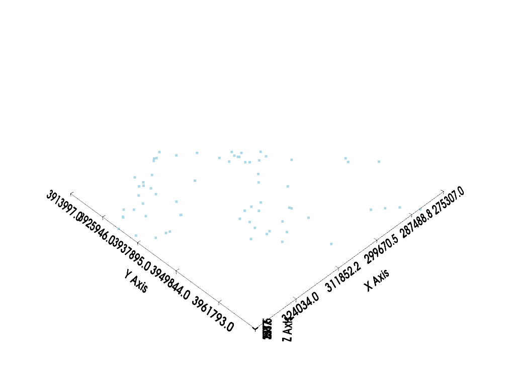
Visualizing the Borehole Collars
Once we have the borehole collars data, we can visualize them in 3D using the pyvista package. This gives us a good overview of where the boreholes are located in space. In this visualization, each borehole will be represented by a point, and we will label the boreholes using their IDs.
well_mesh = to_pyvista_points(collars.collar_loc)

# Plot the collar points
pv_plot([well_mesh], image_2d=False)
<pyvista.plotting.plotter.Plotter object at 0x7f582135f250>
Reading Borehole Survey Data
Borehole surveys give us information about the trajectory of each borehole, including its depth (measured depth). The survey data allows us to compute the full 3D path of each wellbore. We will use the read_survey function from subsurface to read this data.
Create the Survey object
survey_df: pd.DataFrame = read_survey(
    GenericReaderFilesHelper(
        file_or_buffer=raw_borehole_data_csv,
        index_col="name",
        usecols=["name", "md"]
    )
)

survey: Survey = Survey.from_df(survey_df)

survey
Survey(ids=['11', '33XX', 'API_BartellXX', 'Amalgamated_Happold2', 'Arkelian23_26', 'BALD_EAGLE74', 'Bellevue_Deep1', 'Bergman_Trust1', 'Bishop_FeeXX', 'Bishop_FeeXXX', 'CURRY1', 'CallowayXX', 'Cities_Service_TennecoXX', 'Davies1', 'DearingerXX', 'Del_Fortuna1', 'Famosa12_1', 'Golden_State_VintnersXX', 'Gow1', 'HayesXX', 'Helbling1', 'Ingram13_73', 'JewettaXX', 'KCL12', 'KCL15', 'KCL87_25', 'KCL_1144', 'KCL_A58_8', 'KCL_B45', 'KCL_G1', 'Kern_AXX', 'KerncoXX', 'KerrXX', 'Kimberlina1', 'Kramer1', 'Kuhn81_15', 'Law_et_alXX', 'MARQUIS1', 'McCulloch_Camp_et_al1_36', 'Mobil_Pan_Pet_KCL86_35', 'Mobil_Pan_Petroleum_KCL31_15', 'PACIFIC_STATESXX', 'R.A._Shafter_A1', 'RUSSELLXX', 'Roberts_Cox23_1', 'Roe3', 'RoeXX', 'Russell1', 'SUPERIOR_TENNECO_GAUTXX', 'S_&_D_Killingwoth_EPM1', 'Sharples_Marathon_BillingtonXX', 'Shell_Magee_GlideXX', 'St._Anthony1', 'Steele_Petroleum_Co4_1', 'TWIXX', 'TennecoXX', 'Tenneco_Ladd_Rio_Bravo_North87', 'Tenneco_Rio_Bravo32', 'Tenneco_Sun11x_31', 'Tidewater_Capital_Co.XX', 'USLXX', 'USLXXX', 'Union_Tribe_BXX', 'West_Rio_Bravo1', 'Westates44', 'Wiedman55_26', 'Wright_Bloemer74', 'XX32_15', 'XXXX'], survey_trajectory=<subsurface.core.structs.unstructured_elements.line_set.LineSet object at 0x7f57801878c0>, well_id_mapper={'11': 0, '33XX': 1, 'API_BartellXX': 2, 'Amalgamated_Happold2': 3, 'Arkelian23_26': 4, 'BALD_EAGLE74': 5, 'Bellevue_Deep1': 6, 'Bergman_Trust1': 7, 'Bishop_FeeXX': 8, 'Bishop_FeeXXX': 9, 'CURRY1': 10, 'CallowayXX': 11, 'Cities_Service_TennecoXX': 12, 'Davies1': 13, 'DearingerXX': 14, 'Del_Fortuna1': 15, 'Famosa12_1': 16, 'Golden_State_VintnersXX': 17, 'Gow1': 18, 'HayesXX': 19, 'Helbling1': 20, 'Ingram13_73': 21, 'JewettaXX': 22, 'KCL12': 23, 'KCL15': 24, 'KCL87_25': 25, 'KCL_1144': 26, 'KCL_A58_8': 27, 'KCL_B45': 28, 'KCL_G1': 29, 'Kern_AXX': 30, 'KerncoXX': 31, 'KerrXX': 32, 'Kimberlina1': 33, 'Kramer1': 34, 'Kuhn81_15': 35, 'Law_et_alXX': 36, 'MARQUIS1': 37, 'McCulloch_Camp_et_al1_36': 38, 'Mobil_Pan_Pet_KCL86_35': 39, 'Mobil_Pan_Petroleum_KCL31_15': 40, 'PACIFIC_STATESXX': 41, 'R.A._Shafter_A1': 42, 'RUSSELLXX': 43, 'Roberts_Cox23_1': 44, 'Roe3': 45, 'RoeXX': 46, 'Russell1': 47, 'SUPERIOR_TENNECO_GAUTXX': 48, 'S_&_D_Killingwoth_EPM1': 49, 'Sharples_Marathon_BillingtonXX': 50, 'Shell_Magee_GlideXX': 51, 'St._Anthony1': 52, 'Steele_Petroleum_Co4_1': 53, 'TWIXX': 54, 'TennecoXX': 55, 'Tenneco_Ladd_Rio_Bravo_North87': 56, 'Tenneco_Rio_Bravo32': 57, 'Tenneco_Sun11x_31': 58, 'Tidewater_Capital_Co.XX': 59, 'USLXX': 60, 'USLXXX': 61, 'Union_Tribe_BXX': 62, 'West_Rio_Bravo1': 63, 'Westates44': 64, 'Wiedman55_26': 65, 'Wright_Bloemer74': 66, 'XX32_15': 67, 'XXXX': 68})
Reading Lithology Data
Next, we will read the lithology data. Lithology logs describe the rock type or geological unit encountered at different depths within each borehole. Using read_lith, we will extract the lithology data, which includes the top and base depths of each geological formation within the borehole, as well as the formation name.
Your code here:
lith = read_lith(
    GenericReaderFilesHelper(
        file_or_buffer=raw_borehole_data_csv,
        usecols=['name', 'top', 'base', 'formation'],
        columns_map={
            'top': 'top',
            'base': 'base',
            'formation': 'component lith',
        }
    )
)

# Update survey data with lithology information
survey.update_survey_with_lith(lith)

lith
('cell',) are not coordinates with an index xarray dataset must include 'cell' key (KeyError) or xarray 'cell' has no index (ValueError).
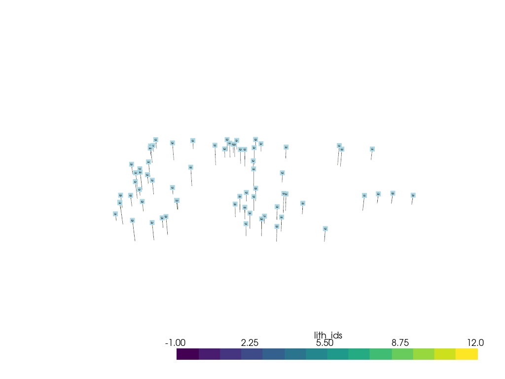
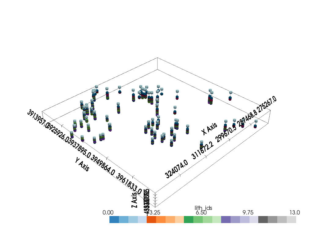
Creating a Borehole Set and Visualizing in 3D
Now that we have both the collar data and the lithology logs, we can combine them into a BoreholeSet object. This object combines the collar, survey, and lithology data and allows us to create a 3D visualization of the borehole trajectories and their associated lithologies.
We will use pyvista to plot the borehole trajectories as lines, and we will color them according to their lithologies. Additionally, we will label the collars for easy identification.
# Combine collar and survey into a BoreholeSet
borehole_set = BoreholeSet(
    collars=collars,
    survey=survey,
    merge_option=MergeOptions.INTERSECT
)
Visualize boreholes with pyvista
import matplotlib.pyplot as plt

well_mesh = to_pyvista_line(
    line_set=borehole_set.combined_trajectory,
    active_scalar="lith_ids",
    radius=40
)

p = init_plotter()

# Set colormap for lithologies
boring_cmap = plt.get_cmap(name="viridis", lut=14)
p.add_mesh(well_mesh, cmap=boring_cmap)

collar_mesh = to_pyvista_points(collars.collar_loc)

p.add_mesh(collar_mesh, render_points_as_spheres=True)
p.add_point_labels(
    points=collars.collar_loc.points,
    labels=collars.ids,
    point_size=10,
    shape_opacity=0.5,
    font_size=12,
    bold=True
)


p.show()
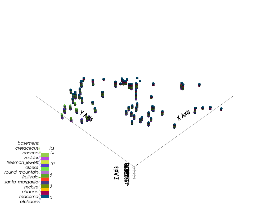
Structural Elements from Borehole Set
Now that we have successfully imported and visualized the borehole data, we can move on to creating the geological formations (or structural elements) based on the borehole data. Each lithological unit will be associated with a unique identifier and a color, allowing us to distinguish between different formations when we visualize the model.
GemPy offers the function gempy.structural_elements_from_borehole_set, which extracts these structural elements from the borehole data and associates each one with a name, ID, and color.
Initialize the color generator for formations
colors_generator = gp.data.ColorsGenerator()

# Define formations and colors
elements = gp.structural_elements_from_borehole_set(
    borehole_set=borehole_set,
    elements_dict={
        "Basement": {
            "id": 1,
            "color": next(colors_generator)
        },
        "etchgoin": {
            "id": 5,
            "color": next(colors_generator)
        },
        "macoma": {
            "id": 8,
            "color": next(colors_generator)
        },
        "chanac": {
            "id": 2,
            "color": next(colors_generator)
        },
        "mclure": {
            "id": 9,
            "color": next(colors_generator)
        },
        "santa_margarita": {
            "id": 12,
            "color": next(colors_generator)
        },
        "fruitvale": {
            "id": 7,
            "color": next(colors_generator)
        },
        "round_mountain": {
            "id": 11,
            "color": next(colors_generator)
        },
        "olcese": {
            "id": 10,
            "color": next(colors_generator)
        },
        "freeman_jewett": {
            "id": 6,
            "color": next(colors_generator)
        },
        "vedder": {
            "id": 14,
            "color": next(colors_generator)
        },
        "eocene": {
            "id": 4,
            "color": next(colors_generator)
        },
        "cretaceous": {
            "id": 3,
            "color": next(colors_generator)
        },
    }
)
Initializing the GemPy Model
After defining the geological formations, we need to initialize the GemPy model. The first step in this process is to create a GeoModel object, which serves as the core container for all data related to the geological model.
We will also define a regular grid to interpolate the geological layers. GemPy uses a meshless interpolator to create geological models in 3D space, but grids are convenient for visualization and computation.
GemPy supports various grid types, such as regular grids for visualization, custom grids, topographic grids, and more. For this example, we will use a regular grid with a medium resolution.
import gempy_viewer as gpv

# Create a structural group with the elements
group = gp.data.StructuralGroup(
    name="Stratigraphic Pile",
    elements=elements,
    structural_relation=gp.data.StackRelationType.ERODE
)

# Define the structural frame
structural_frame = gp.data.StructuralFrame(
    structural_groups=[group],
    color_gen=colors_generator
)
Defining Model Extent and Grid Resolution
We now determine the extent of our model based on the surface points provided. This ensures that the grid covers the entire area where the geological data points are located. Additionally, we set a grid resolution of 50x50x50 for a balance between performance and model detail.
all_surface_points_coords: gp.data.SurfacePointsTable = structural_frame.surface_points_copy
extent_from_data = all_surface_points_coords.xyz.min(axis=0), all_surface_points_coords.xyz.max(axis=0)
# Initialize GeoModel
geo_model = gp.data.GeoModel.from_args(
    name="Stratigraphic Pile",
    structural_frame=structural_frame,
    grid=gp.data.Grid(
        extent=[extent_from_data[0][0], extent_from_data[1][0], extent_from_data[0][1], extent_from_data[1][1], extent_from_data[0][2], extent_from_data[1][2]],
        resolution=(50, 50, 50)
    ),
    interpolation_options=gp.data.InterpolationOptions.from_args(
        range=5,
        c_o=10,
        mesh_extraction=True,
        number_octree_levels=3,
    ),
)
3D Visualization of the Model
After initializing the GeoModel, we can proceed to visualize it in 3D using GemPy’s plot_3d function. This function allows us to see the full 3D geological model with all the defined formations.
gempy_plot = gpv.plot_3d(
    model=geo_model,
    kwargs_pyvista_bounds={
            'show_xlabels': False,
            'show_ylabels': False,
    },
    show=True,
    image=False
)
Adding Boreholes and Collars to the Visualization
To enhance the 3D model, we can combine the geological formations with the borehole trajectories and collar points that we visualized earlier. This will give us a complete picture of the subsurface, showing both the lithological units and the borehole paths.
sp_mesh: pyvista.PolyData = gempy_plot.surface_points_mesh

pyvista_plotter = init_plotter()
pyvista_plotter.show_bounds(all_edges=True)

# Set limits for the units to visualize
units_limit = [0, 13]
pyvista_plotter.add_mesh(
    well_mesh.threshold(units_limit),
    cmap="tab20c",
    clim=units_limit
)

# Add collar points
pyvista_plotter.add_mesh(
    collar_mesh,
    point_size=10,
    render_points_as_spheres=True
)

# Label the collars with their names
pyvista_plotter.add_point_labels(
    points=collars.collar_loc.points,
    labels=collars.ids,
    point_size=10,
    shape_opacity=0.5,
    font_size=12,
    bold=True
)
# Add surface points from the geological model
pyvista_plotter.add_actor(gempy_plot.surface_points_actor)

# Show the final 3D plot
pyvista_plotter.show()
Step-by-Step Model Building
When building a geological model, it’s often better to proceed step by step, adding one surface at a time, rather than trying to interpolate all formations at once. This allows for better control over the model and helps avoid potential issues from noisy or irregular data.
Adding Surfaces and Formations
In GemPy, surfaces mark the bottom of each geological unit. For our model, we will add the first two formations along with the basement, which always needs to be defined. After this, we can visualize the surfaces in 2D.
group = gp.data.StructuralGroup(
    name="Stratigraphic Pile Top",
    elements=elements[:3],
    structural_relation=gp.data.StackRelationType.ERODE
)
geo_model.structural_frame.structural_groups[0] = group


# Visualize the surfaces in 2D

g2d = gpv.plot_2d(geo_model)
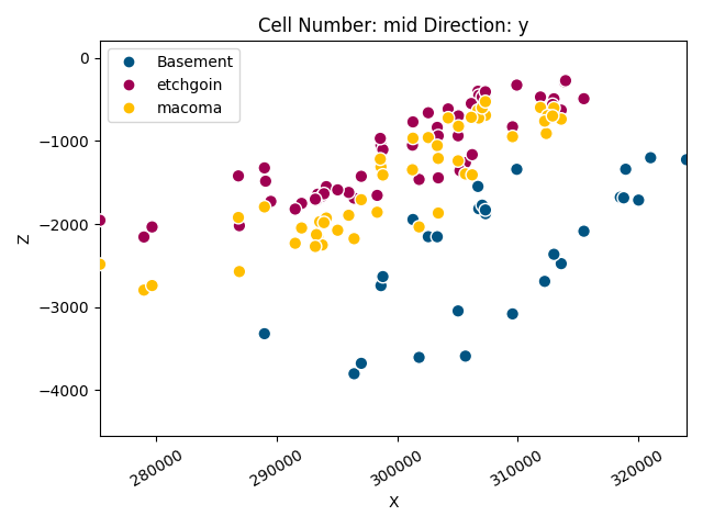
g2d.fig
<Figure size 640x480 with 1 Axes>
Minimum Input Data for Interpolation
To interpolate the geological layers, GemPy requires at least:
Two surface points per geological unit
One orientation measurement per series
Let’s add an orientation for one of the units.
gp.add_orientations(
    x=[300000],
    y=[3930000],
    z=[0],
    elements_names=elements[0].name,
    pole_vector=np.array([0, 0, 1]),
    geo_model=geo_model
)
Model Computation
Now that we have the necessary surface points and orientations, we can compute the final geological model. The compute_model function will take all the input data and perform the interpolation to generate the 3D subsurface structure.
geo_model.interpolation_options
InterpolationOptions(kernel_options=KernelOptions(range=5.0, c_o=10.0, uni_degree=1, i_res=4.0, gi_res=2.0, number_dimensions=3, kernel_function=AvailableKernelFunctions.cubic, kernel_solver=Solvers.DEFAULT, compute_condition_number=False, optimizing_condition_number=False, condition_number=None), evaluation_options=EvaluationOptions(_number_octree_levels=3, _number_octree_levels_surface=4, octree_curvature_threshold=-1.0, octree_error_threshold=1.0, octree_min_level=2, mesh_extraction=True, mesh_extraction_masking_options=<MeshExtractionMaskingOptions.INTERSECT: 3>, mesh_extraction_fancy=True, evaluation_chunk_size=500000, compute_scalar=True, compute_scalar_gradient=False, verbose=False), debug=False, cache_mode=<CacheMode.IN_MEMORY_CACHE: 3>, cache_model_name='Stratigraphic Pile', block_solutions_type=<BlockSolutionType.DENSE_GRID: 2>, sigmoid_slope=5000000)
Setting Backend To: AvailableBackends.PYTORCH
GPU requested but unavailable; falling back to CPU (GEMPY_GPU_FALLBACK=True)
Setting Backend To: AvailableBackends.PYTORCH
Chunking done: 42 chunks
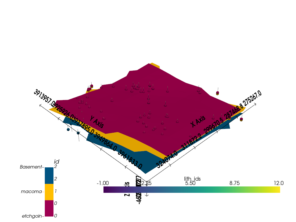
Final 3D Visualization
Let’s take a look at the final model, combining the borehole data and geological formations in 3D.
g3d = gpv.plot_3d(geo_model, show_lith=False, show=False)
g3d.p.add_mesh(well_mesh)
g3d.p.show()
Conclusion
In this tutorial, we have demonstrated how to take borehole data and create a 3D geological model in GemPy. We explored how to extract structural elements from borehole data, set up a regular grid for interpolation, and visualize the resulting model in both 2D and 3D.
GemPy’s flexibility allows you to iteratively build models and refine your inputs for more accurate results, and it integrates seamlessly with borehole data for subsurface geological modeling.
For further reading and resources, check out:
Extra Resources
Page: https://www.gempy.org/
Paper: https://www.gempy.org/theory
Further training and collaborations
https://www.terranigma-solutions.com/
Total running time of the script: (0 minutes 2.291 seconds)